Download
1 / 22
220 likes | 322 Vues
Distributed Computation of the Mode. Fabian Kuhn Thomas Locher ETH Zurich, Switzerland Stefan Schmid TU Munich, Germany. TexPoint fonts used in EMF. Read the TexPoint manual before you delete this box.: A A A A A A A A. Internet. General Trend in Information Technology.

E N D
Distributed Computationof the Mode Fabian KuhnThomas LocherETH Zurich, Switzerland Stefan SchmidTU Munich, Germany TexPoint fonts used in EMF. Read the TexPoint manual before you delete this box.: AAAAAAAA
Internet General Trend in Information Technology CentralizedSystems NetworkedSystems Large-scaleDistributed Systems New Applications andSystem Paradigms
Distributed Data • Earlier: Data stored on a central sever • Today: Data distributedover network(e.g. distributed databases, sensor networks) • Typically: Data stored where it occurs • Nevertheless: Need to query all / large portion of data • Methods for distributed aggregation needed
Model • Network given by a graph G=(V,E) • Nodes: Network devices, Edges: Communication links • Data stored at the nodes • For simplicity: each node has exactly one data item / value • Query initiated at some node • Compute result of query by sending around (small) messages
Simple Aggregation Functions • Simple aggregation functions: 1convergecaston spanning tree(simple: algebraic, distributive e.g.: min, max, sum, avg, …) • On BFS tree: time complexity = O(D) (D = diameter) • k independent simple functions:Time O(D+k) by using pipelining
The Mode • Mode = most frequent element • Every node has an element from {1,…,K} • k different elementse1,…,ek, frequencies: m1¸m2¸ … ¸mk(k and mi are not known to algorithm) • Goal: Find mode = element occuringm1 times • Per message: 1 element, O(log n + log K) additional bits
Mode: Simple Algorithm • Send all elements to root, aggregate frequencies along the way • Using pipelining, time O(D+k) • Always send smallest element first to avoid empty queues • For almost uniform frequency distributions, algorithm is optimal • Goal: Fast algorithm if frequency distribution is good (skewed)
Mode: Basic Idea • Assume, nodes have access to common random hash functionsh1, h2, … where hi: {1,…,K} {-1,+1} • Apply hi to all elements: element e3, hi(e3)=+1 element e2, hi(e2)=+1 element e4, hi(e4)=-1 element e5, hi(e5)=-1 element e1, hi(e1)=-1 hi … -1 +1 … m4 m1 m5 m3 m2
Mode: Basic Idea • Intuition: bin containing mode tends to be larger • Introduce counter cifor each element ei • Go through hash functions h1, h2, … • Function hj: Increment ciby number of elements in bin hj(ei) • Intuition: counter c1of mode will be largest after some time
Compare Counters • Compare counters c1 and c2 of elements e1 and e2 • If hj(e1) = hj(e2), c1 and c2 increased by same amount • Consider only j for which hj(e1) hj(e2) • Change in c1 – c2 difference: where
Counter Difference • Given indep. Z1, …, Zn, Pr(Zi=®i)=Pr(Zi=-®i)=1/2 • Chernoff: • H: set of hash function with hj(e1) hj(e2), |H|=s
Counter Difference • is called the 2nd frequency moment • Can make the same for all other counters: • If hj(e1) hj(ei) for s hash fct.: • hj(e1) hj(ei) for roughly 1/2 of all hash functions • After considering O(F2/(m1–m2)2¢log n) hash functions: c1 largest counter w.h.p.
Distributed Implementation • Assume, nodes know hash functions • Bin sizes for each hash function: time O(D) (simply a sum) • Update counter in time O(D) (root broadcasts bin sizes) • We can pipeline computations for different hash functions • Algorithm with time complexity: • … only good if m1-m2 large
Improvement • Only apply algorithm until w.h.p., c1 > ci if m1¸ 2mi • Time: • Apply simple deterministic algorithm for remaining elements • #elementsei with m1¸2mi: at most 4F2/m12 • Time of second phase:
Improved Algorithm • Many details missing (in particular: need to know F2, m1) • Can be done (F2: use ideas from [Alon,Matias,Szegedy 1999]) • If nodes have access to common random hash functions:Mode can be computed in time
Random Hash Functions • Still need mechanism that provides random hash functions • Select functions in advance (hard-wired into alg): algorithm does not work for all input distributions • Choosing random hash function h : [K] {-1,+1} requires sending O(K) bits we want messages of size O(log K + log n)
Quasi-Random Hash Functions • Fix set H of hash functions s.t. |H|= O(poly(n,K)) such that H satisfies a set of uniformity conditions • Choosing random hash function from H requires onlyO(log n + log K) bits. • Show that algorithm still works if hash functions are from a set H that satisfies uniformity conditions
Quasi-Random Hash Functions • Possible to give a set of uniformity conditions that allow to prove that algorithm still works (quite involved…) • Using probabilistic method:Show that a set H of size O(poly(n,K)) satisfying uniformity conditions exists.
Distributed Computation of the Mode • Lower bound based on generalization (by Alon et. al.) of set disjointness communication complexity lower bound by Razborov Theorem: The mode can be computed in time O(D+F2/m12¢log n) by a distributed algorithm. Theorem: The time needed to compute the mode by a distributed algorithm is at least (D+F5/(m15¢log n)).
Related Work • Paper by Charikar, Chen, Farach-Colton:Finds element with frequency (1-²)¢m1 in a streaming model with a different method • It turns out: • Basic techniques of Charikar et. al. can be applied in distributed case • Our techniques can be applied in streaming model • Both techniques yield same results in both cases
Conclusions: • Obvious open problem:Close gap between upper and lower bound • We believe: Upper bound is tight • Proving that upper bound is tight would probably also prove a conjecture in [Alon,Matias,Szegedy 1999] regarding the space complexity of the computation of frequency moments in streaming models.