Download
1 / 1
10 likes | 110 Vues
NDVI and quality data. 1. S tack the NDVI and quality data, respectively. MODIS NDVI growing season metrics for Alaska: Product development and monitoring applications J. Zhu 1 , A.E. Miller 2 , P . Martyn 2 , D. Broderson 1 , and T. Heinrichs 1

E N D
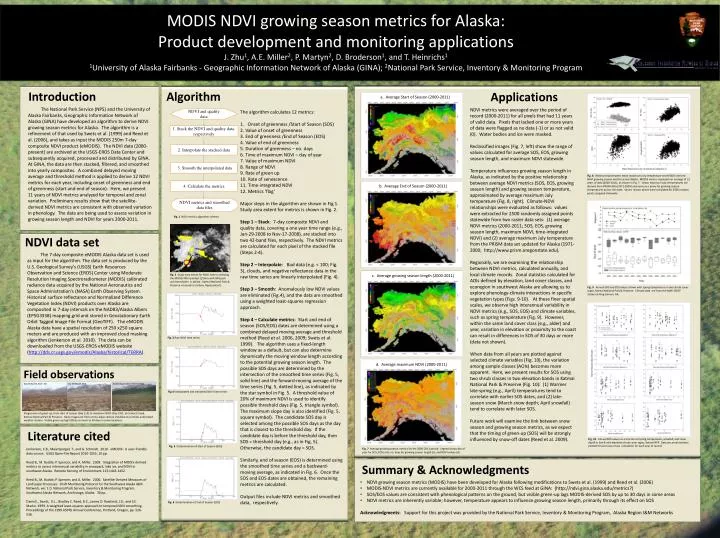
NDVI and quality data 1. Stack the NDVI and quality data, respectively MODIS NDVI growing season metrics for Alaska: Product development and monitoring applications J. Zhu1, A.E. Miller2, P. Martyn2, D. Broderson1, and T. Heinrichs1 1University of Alaska Fairbanks - Geographic Information Network of Alaska (GINA); 2National Park Service, Inventory & Monitoring Program 2. Interpolate the stacked data 3. Smooth the interpolated data Introduction 4. Calculate the metrics Algorithm NDVI metrics and smoothed data files Introduction Algorithm Applications a. Average Start of Season (2000-2011) The National Park Service (NPS) and the University of Alaska Fairbanks, Geographic Information Network of Alaska (GINA) have developed an algorithm to derive NDVI growing season metrics for Alaska. The algorithm is a refinement of that used by Swets et al. (1999) and Reed et al. (2006), and takes as input the MODIS 250m 7-day composite NDVI product (eMODIS). The NDVI data (2000-present) are archived at the USGS-EROS Data Center and subsequently acquired, processed and distributed by GINA. At GINA, the data are then stacked, filtered, and smoothed into yearly composites. A combined delayed moving average and threshold method is applied to derive 12 NDVI metrics for each year, including onset of greenness and end of greenness (start and end of season). Here, we present 11 years of NDVI metrics analyzed for temporal and zonal variation. Preliminary results show that the satellite-derived NDVI metrics are consistent with observed variation in phenology. The data are being used to assess variation in growing season length and NDVI for years 2000-2011. NDVI metrics were averaged over the period of record (2000-2011) for all pixels that had 11 years of valid data. Pixels that lacked one or more years of data were flagged as no data (-1) or as not valid (0). Water bodies and ice were masked. Reclassified images (Fig. 7, left) show the range of values calculated for average SOS, EOS, growing season length, and maximum NDVI statewide. Temperature influences growing season length in Alaska, as indicated by the positive relationship between average NDVI metrics (SOS, EOS, growing season length) and growing season temperature, approximated by average maximum July temperature (Fig. 8, right). Climate-NDVI relationships were evaluated as follows: values were extracted for 2500 randomly assigned points statewide from two raster data sets: (1) average NDVI metrics (2000-2011; SOS, EOS, growing season length, maximum NDVI, time-integrated NDVI) and (2) average maximum July temperature from the PRISM data set updated for Alaska (1971-2000; http://www.prism.oregonstate.edu). Regionally, we are examining the relationship between NDVI metrics, calculated annually, and local climate records. Zonal statistics calculated for AOIs defined by elevation, land cover classes, and ecoregion in southwest Alaska are allowing us to explore phenology-climate interactions in specific vegetation types (Figs. 9-10). At these finer spatial scales, we observe high interannual variability in NDVI metrics (e.g., SOS, EOS) and climate variables, such as spring temperature (Fig. 9). However, within the same land cover class (e.g., alder) and year, variation in elevation or proximity to the coast can result in differences in SOS of 30 days or more (data not shown). When data from all years are plotted against selected climate variables (Fig. 10), the variation among sample classes (AOIs) becomes more apparent. Here, we present results for SOS using two shrub classes in two elevation bands in Katmai National Park & Preserve (Fig. 10): (1) Warmer late-spring (e.g., April) temperatures tend to correlate with earlier SOS dates, and (2) late-season snow (March snow depth; April snowfall) tend to correlate with later SOS. Future work will examine the link between snow season and growing season metrics, as we expect that the timing of green-up (SOS) will be strongly influenced by snow-off dates (Reed et al. 2009). The algorithm calculates 12 metrics: Onset of greenness /Start of Season (SOS) 2. Value of onset of greenness 3. End of greenness /End of Season (EOS) 4. Value of end of greenness 5. Duration of greenness – no. days 6. Time of maximum NDVI – day of year 7. Value of maximum NDVI 8. Range of NDVI 9. Rate of green up 10. Rate of senescence 11. Time-integrated NDVI 12. Metrics ‘flag’ Major steps in the algorithm are shown in Fig 1. Study area extent for metrics is shown in Fig. 2. Step 1 – Stack: 7-day composite NDVI and quality data, covering a one year time range (e.g., Jan-29-2008 to Nov-17-2008), are stacked into two 42-band files, respectively. The NDVI metrics are calculated for each pixel of the stacked file (Steps 2-4). Step 2 – Interpolate: Bad data (e.g. < 100; Fig. 3), clouds, and negative reflectance data in the raw time series are linearly interpolated (Fig. 4). Step 3 – Smooth: Anomalously low NDVI values are eliminated (Fig.4), and the data are smoothed using a weighted least-squares regression approach. Step 4 – Calculate metrics: Start and end of season (SOS/EOS) dates are determined using a combined delayed moving average and threshold method (Reed et al. 2006, 2009; Swets et al. 1999). The algorithm uses a fixed-length window as a default, but can also determine dynamically the moving window length according to the potential growing season length. The possible SOS days are determined by the intersection of the smoothed time series (Fig. 5, solid line) and the forward-moving average of the time series (Fig. 5, dotted line), as indicated by the star symbol in Fig. 5. A threshold value of 20% of maximum NDVI is used to identify possible threshold days (Fig. 5, triangle symbol). The maximum slope day is also identified (Fig. 5, square symbol). The candidate SOS day is selected among the possible SOS days as the day that is closest to the threshold day. If the candidate day is before the threshold day, then SOS = threshold day (e.g., as in Fig. 5). Otherwise, the candidate day = SOS. Similarly, end of season (EOS) is determined using the smoothed time series and a backward-moving average, as indicated in Fig. 6. Once the SOS and EOS dates are obtained, the remaining metrics are calculated. Output files include NDVI metrics and smoothed data, respectively. Fig. 8 Relationship between mean maximum July temperature and MODIS-derived NDVI growing season metrics across Alaska. MODIS metrics represent an average of 12 years of data (2000-2011), as shown in Fig. 7. Mean maximum July temperatures are derived from PRISM data (1971-2000) and serve as a proxy for growing season temperatures across the state. Values shown above were calculated for 2500 random points assigned statewide. b. Average End of Season (2000-2011) Fig. 1 NDVI metrics algorithm schema NDVI data set The 7-day composite eMODISAlaska data set is used as input for the algorithm. The data set is produced by the U.S. Geological Survey’s (USGS) Earth Resources Observation and Science (EROS) Center using Moderate Resolution Imaging Spectroradiometer(MODIS) calibrated radiance data acquired by the National Aeronautics and Space Administration’s (NASA) Earth Observing System. Historical surface reflectance and Normalized Difference Vegetation Index (NDVI) products over Alaska are composited in 7-day intervals on the NAD83/Alaska Albers (EPSG3338) mapping grid and stored in Geostationary Earth Orbit Tagged Image File Format (GeoTIFF). The eMODIS Alaska data have a spatial resolution of 250 x250 square meters and are produced with an improved cloud masking algorithm (Jenkerson et al. 2010). The data can be downloaded from the USGS-EROS eMODISwebsite (http://dds.cr.usgs.gov/emodis/Alaska/historical/TERRA). • Fig. 2 Study area extent for NDVI metrics showing the MODIS NDVI product (250m) with NPS park unit boundaries in yellow. Katmai National Park & Preserve is bound in red (see ‘Applications’). c. Average growing season length (2000-2011) Fig. 9 Annual SOS and EOS values shown with spring temperature in two shrub cover types, Katmai National Park & Preserve. Climate data are from the NWS-COOP station at King Salmon, AK. Fig. 3 Raw NDVI time series d. Average maximum NDVI (2000-2011) Field observations Day 119 (April 29, 2011) – SOS Day 149 (May 29, 2011) Day 232 (Aug 20, 2011) – Maximum NDVI Fig.4 Interpolated and smoothed NDVI time series Progression of green-up, from start of season (Day 119) to maximum NDVI (Day 232), at Contact Creek, Katmai National Park & Preserve. Daily images are from a time-lapse camera installed at a remote automated weather station. Visible green-up lags SOS by as much as 30 days in some locations. Literature cited Fig. 10 Annual SOS values as a function of spring temperature, snowfall, and snow depth in low & mid-elevation shrub cover types, Katmai NPP. Data are zonal statistics plotted for land cover class x elevation for each year of record. Fig. 5 Determination of Start of Season (SOS) Jenkerson, C.B., Maiersperger, T., and G. Schmidt. 2010. eMODIS: A user-friendly data source. USGS Open-File Report 2010-1055, 10 pp. Reed B., M. Budde, P. Spencer, and A. Miller. 2009. Integration of MODIS-derived metrics to assess interannual variability in snowpack, lake ice, and NDVI in southwest Alaska. Remote Sensing of Environment 113:1443-1452. Reed B., M. Budde, P. Spencer, and A. Miller. 2006. Satellite-Derived Measures of Landscape Processes: Draft Monitoring Protocol for the Southwest Alaska I&M Network, ver. 1.0. National Park Service, Inventory & Monitoring Program, Southwest Alaska Network, Anchorage, Alaska. 30 pp. Daniel L. Swets, D.L., Bradley C. Reed, B.C., James D. Rowland, J.D., and S.E. Marko. 1999. A weighted least-squares approach to temporal NDVI smoothing. Proceedings of the 1999 ASPRS Annual Conference, Portland, Oregon, pp. 526-536. Fig. 7 Average growing season metrics for the 2000-2011 period. Legend shows day of year for SOS, EOS (a-b); no. days for growing season length (c); and NDVIvalues (d). Summary & Acknowledgments • NDVI growing season metrics (MODIS) have been developed for Alaska following modifications to Swets et al. (1999) and Reed et al. (2006) • MODIS-NDVI metrics are currently available for 2000-2011 through the WCS feed at GINA: (http://ndvi.gina.alaska.edu/metrics?) • SOS/EOS values are consistent with phenological patterns on the ground, but visible green-up lags MODIS-derived SOS by up to 30 days in some areas • NDVI metrics are inherently variable; however, temperature appears to influence growing season length, primarily through its effect on SOS • Acknowledgments: Support for this project was provided by the National Park Service, Inventory & Monitoring Program, Alaska Region I&M Networks Fig. 6 Determination of End of Season (EOS)