Download
1 / 21
210 likes | 345 Vues
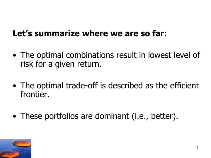
Let’s summarize where we are so far: The optimal combinations result in lowest level of risk for a given return. The optimal trade-off is described as the efficient frontier. These portfolios are dominant (i.e., better). Including Riskless Investments. The optimal combination becomes linear

E N D
Let’s summarize where we are so far: The optimal combinations result in lowest level of risk for a given return. The optimal trade-off is described as the efficient frontier. These portfolios are dominant (i.e., better).
Including Riskless Investments The optimal combination becomes linear A single combination of risky and riskless assets will dominate 6-2
CAL (P) CAL (A) E(rP&F) E(rP) CAL (Global minimum variance) E(rA) A G P P&F ALTERNATIVE CALS E(r) Efficient Frontier P F Risk Free s A 6-3
The Capital Market Line or CML CAL (P) = CML E(r) Efficient Frontier E(rP&F) • The optimal CAL is called the Capital Market Line or CML • The CML dominates the EF P E(rP) E(rP&F) F Risk Free s P&F P P&F 6-4
Dominant CAL with a Risk-Free Investment (F) CAL(P) = Capital Market Line or CML dominates other lines because it has the the largest slope Slope = (E(rp) - rf) / sp (CML maximizes the slope or the return per unit of risk or it equivalently maximizes the Sharpe ratio) We want our CAL to be drawn tangent to the Efficient Frontier and the risk-rate. This tells us the “optimal risky portfolio”. Once we’ve drawn the CAL, we can use the investor’s risk-aversion to determine where he or she should be on the CAL. 6-5
Capital Allocation Line and Investor Risk Aversion Assume that for the “optimal risky portfolio”: E(rp) =15%, σp = 22%, and rf = 7%. Each investor’s “complete portfolio” (we’ll use subscript “C” to designate it) is determined by their risk aversion. Let “y” be the fraction of the dollars they invest in the optimal risky portfolio and “1-y” equal the fraction in T-bills. Expected reward, risk, and Sharpe measure for each investor’s “complete portfolio”: E(rc) = (1- y) rf + (y) E(rp) σc = y σp S = (E(rp) - rf ) / σp y 1-y E(rc) – rfsc S Retiree Fred 0 1.0 0 0 ? Mid-life Rose 0.5 0.5 (.5)(8%) = 4% 11% 8/22 The Just-Married Jones 1.0 0.0 8% 22% 8/22 “Single and Loving it” Sali * 1.4 - 0.4 (1.4)(8%) =11.2% 30.8% 8/22 Doubling the risk, doubles the expected reward. Sharpe ratio doesn’t change.
Capital Allocation Line and Investor Risk Aversion Here is the Capital Allocation Line for the example: E(rp) =15%, σp = 22%, and rf = 7%. Optimal risky portfolio is point “P” Sali (y=1.4) Fred (y=0) Just-Married Jones (y=1.0) Rose (y=.5) The Capital Allocation Line has an intercept of rf and a slope (rise/run) equal to the Sharpe ratio.
Individual securities We have learned that investors should diversify. Individual securities will be held in a portfolio. What do we call the risk that cannot be diversified away, i.e., the risk that remains when the stock is put into a portfolio? How do we measure a stock’s systematic risk? Consequently, the relevant risk of an individual security is the risk that remains when the security is placed in a portfolio. Systematic risk 6-9
Systematic risk Systematic risk arises from events that effect the entire economy such as a change in interest rates or GDP or a financial crisis such as occurred in 2007and 2008. If a well diversified portfolio has no unsystematic risk then any risk that remains must be systematic. That is, the variation in returns of a well diversified portfolio must be due to changes in systematic factors. 6-10
Individual securities How do we measure a stock’s systematic risk? Systematic Factors Returns well diversifiedportfolio Δ interest rates, Δ GDP, Δ consumer spending, etc. Returns Stock A 6-11
Risk Premium Format Let: Ri = (ri - rf) Risk premium format Rm = (rm - rf) The Model: Ri = ai + ßi(Rm)+ ei 6-12
Single Factor Model Ri = E(Ri) + ßiM + ei Ri = Actual excess return = ri – rf E(Ri) = expected excess return Two sources of Uncertainty M ßi ei = some systematic factor or proxy; in this case M is unanticipated movement in a well diversified broad market index like the S&P500 = sensitivity of a securities’ particular return to the factor = unanticipated firm specific events 6-13
Single Index Model Parameter Estimation Market Risk Prem Risk Prem or Index Risk Prem αi = the stock’s expected excess return if the market’s excess return is zero, i.e., (rm - rf) = 0 ßi(rm - rf)= the component of excess return due to movements in the market index ei = firm specific component of excess return that is not due to market movements 6-14
Estimating the Index Model Security Characteristic Line Scatter Plot Excess Returns (i) . . . . . . . . . . . . . . . . . . . . . . . . . . Excess returns on market index . . . . . . . . . . . . . . . . . . . . . . . . Ri = ai + ßiRm + ei Slope of SCL = beta y-intercept = alpha 6-15
Components of Risk Market or systematic risk: Unsystematic or firm specific risk: Total risk = ßiM + ei risk related to the systematic or macro economic factorin this case the market index risk not related to the macro factor or market index Systematic + Unsystematic i2 = Systematic risk + Unsystematic Risk 6-16
Measuring Components of Risk si2 = where; bi2sm2 + s2(ei) si2 = total variance bi2sm2 = systematic variance s2(ei) = unsystematic variance 6-17
Total Risk = Systematic Risk / Total Risk = Examining Percentage of Variance Systematic Risk + Unsystematic Risk r2 ßi2 sm2 / si2 = r2 bi2sm2 / (bi2sm2 + s2(ei)) = r2 6-18
Advantages of the Single Index Model Reduces the number of inputs needed to account for diversification benefits If you want to know the risk of a 25 stock portfolio you would have to calculate 25 variances and (25x24) = 600 covariance terms With the index model you need only 25 betas Easy reference point for understanding stock risk. βM = 1, so if βi > 1 what do we know? If βi < 1? 6-19
Sharpe Ratios and alphas When ranking portfolios and security performance we must consider both return & risk “Well performing” diversified portfolios provide high Sharpe ratios: Sharpe = (rp – rf) / p You can also use the Sharpe ratio to evaluate an individual stock if the investor does not diversify 6-20
Sharpe Ratios and alphas “Well performing” individual stocks held in diversified portfolios can be evaluated by the stock’s alpha in relation to the stock’s unsystematic risk. 6-21