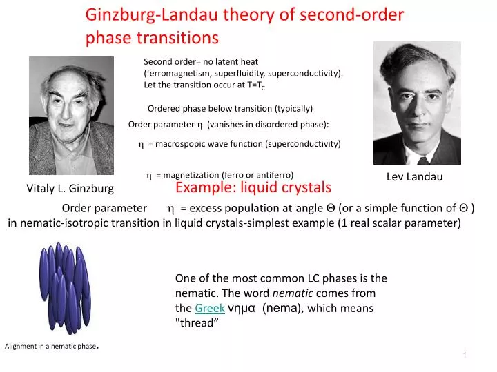
Ginzburg-Landau theory of second-order phase transitions

1. Ginzburg-Landau theory of second-order phase transitions Second order= no latent heat (ferromagnetism, superfluidity, superconductivity). Let the transition occur at T=TC Ordered phase below transition (typically) Order parameter h (vanishes in disordered phase): h = macrospopic wave function (superconductivity) h = magnetization (ferro or antiferro) Lev Landau Vitaly L. Ginzburg Example: liquid crystals Order parameter h = excess population atangle Q (or a simple function of Q ) in nematic-isotropic transition in liquid crystals-simplest example (1 real scalar parameter) One of the most common LC phases is the nematic. The word nematic comes from the Greekνημα (nema), which means "thread” Alignment in a nematic phase. 1

2. (see lectures by A. Salonen) Tfy-0.3252 Soft Matter Physics, Fall 2009 / E. Salonen 2

3. Equilibrium Condition Gibbs free energy Gibbs free energy must be minimum at equilibrium at any T How G depends on h near the transition Temperature Order parameter h is 0 or small (since it vanishes in disordered phase) Near the transition Gibbs free energy must be minimum at equilibrium in disorderesìd phase Therefore the expansion around critical point starts from second order At h=0 there is a minimum or a maximum 3

4. Above TC minimum at h=0 (order parameter vanishes at equilibrium in disordered phase GL Phenomenological model, with terms up to 4° order: G-G0 At the transition T= TC G must be the same for nematic and isotropic (equilibrium). Below TC maximum at h=0 4

5. Discontinuity of Order Parameter h at Tc One obtains the discontinuity of order parameter by imposing equilibrium and minimum at Tc often written in the form 5

6. Order parameter versus T Above, we got the discontinuity To obtain h(T) we can start from the equilibrium condition One can write T* in terms of TC and the other parameters. The order parameter is discontinuous at transition. Insert h=hc back into G-G0 equation T* 6

7. To get rid of the double sign, choose the right h at the transition: 7

8. Langevin paramagnetism Paul Langevin (1872-1946) 8

9. Weiss mean field theory (1907) of Ferromagnetism: PIERRE-ERNEST WEISS The spontaneous magnetization may remain even for H=0 born March 25, 1865, Mulhouse, France. died Oct. 24, 1940, Lyon, France. One can fix the parameter l in terms of Tc as follows: 9

10. x=y 1 solution if T>Tc, 2 otherwise

11. Spontaneous magnetization for H=0 T Tc from below: From the graphical solution we gain the trend with T of the M(T) curve. Increasing T at H=0 M must vanish, but how? PIERRE-ERNEST WEISS born March 25, 1865, Mulhouse, France. died Oct. 24, 1940, Lyon, France. 11

12. A different experiment: fix T =Tc and measure M dependence on H atfor H0 . Since M is small we can expand 12

13. How do these critical exponents arise? Widom in 1965 put forth the scaling hypothesis for magnetic materials in field B: This produces relations between various critical exponents. The dependence on approximation scheme and dimensionality is dramatic. Behavior for T>Tc , in paramagnetic phase M small

14. (Weiss theory) (Weiss theory) 14

15. Ising Model in 1d , defined on a closed ring (model invented in 1920 by Wilhelm Lenz as a thesis for Ernst Ising) where the sums over sites and sn is a classical spin taking the values +1,-1. The Partition function is defined by: 15

16. Rearrange: 1 2 There is a [ ] factor for each bond; each factor is a matrix product 16

17. 17

18. For H0, 18

19. We need to note that another reasoning is possible. Instead of one can decide to distribute the interactions with H symmetrically among the bonds and define a different transfer matrix, which is also common in textbooks, with elements: 1 1 2 2 This is transfer matrix has the same trace and the same determinant as the previous one, hence the eigenvalues are the same. 19

20. Thermodynamic limit: only large eigenvalue matters The peak in specific heat is due to some short-range order (increasing T at low temperatures spins are reversed and this costs energy). 20

21. no ferromagnetism, no phase transition, no long-range order! 1d theory fails to explain magnetism. Why? For large N there is a gain in F at any T. In 2d is different. 21

22. Rudolf Peierls Centre for Theoretical Physics 1 Keble Road Oxford, OX1 3NP England  22

23. Percolation problem: Renormalization group approach to the onset of conductivity A.P.Young and R.B. Stinchcombe J. Phys. C 8 L535 (1975) Consider a regular lattice (sites connected by bonds, with Z bonds per site) Remove a fraction 1-p of bonds at random. Conductivity is a function of p. There is a critical value pc such that for p< pc the lattice is not conducting and consists of clusters of connected sites in a sea of isolated sites. If we pick two sites far apart the probability of finding a continuous path joining them gets small. Conversely, for p> pc the film as a whole is conducting , even if it contains nonconducting islands. The macroscopic conductivity S of the lattice is a function S=S(p, s), s = bond conductivity . Let us consider a square lattice: Howtofindanapproximationtopc? Byscaling! Forexampe, discardhalfof the x and halfof the y and consider a new lattice where the nodes can beconnected or notwith some probability. The newproblemissimilar. We can exploit that! 23

24. Decimation 24

25. A similar problem can be posed on the lattice with vertices 1,2, .. or with the rescaled lattice A,B,…on a larger square mesh. p1= probability in rescaled network , s1 = bond conductivity in rescaled network S=S(p1, s1) 25

26. By comparison with the exact results one can evaluate approximations.

27. Consider only paths involving a,b,c,d. What is the probability p1 that nodes A and B of new lattice are connected? 1 B b a g C d A 2 D 27

28. 28