Download

1 / 64
640 likes | 821 Vues
Randomized Algorithms and Motif Finding. Outline. Randomized QuickSort Randomized Algorithms Greedy Profile Motif Search Gibbs Sampler Random Projections. Randomized Algorithms. Randomized algorithms make random rather than deterministic decisions.

E N D
Outline • Randomized QuickSort • Randomized Algorithms • Greedy Profile Motif Search • Gibbs Sampler • Random Projections
Randomized Algorithms • Randomized algorithms make random rather than deterministic decisions. • The main advantage is that no input can reliably produce worst-case results because the algorithm runs differently each time. • These algorithms are commonly used in situations where no exact and fast algorithm is known.
Introduction to QuickSort • QuickSort is a simple and efficient approach to sorting: • Select an element m (the pivot) from an unsorted array c and divide the array into two subarrays: csmall - elements smaller than m and clarge- elements larger than m. • Recursively sort the subarrays and combine them together in the sorted array csorted
Example of QuickSort Given an array: c = { 5, 2, 8, 4, 3, 1, 7, 6, 9 } Step 1: Choose the first element as m c = { 6, 3, 2, 8, 4, 5, 1, 7, 0, 9 } Our Selection
Example of QuickSort (cont’d) Step 2: Split the array into csmall and clarge Csmall = { 3, 2, 4, 5, 1, 0 } C = { 6, 3, 2, 8, 4, 5, 1, 7, 0, 9 } Clarge= { 8, 7, 9 }
Example of QuickSort (cont’d) Step 3: Recursively do the same thing to csmalland clargeuntil each subarray has only one element or is empty. Csmall = { 3, 2, 4, 5, 1, 0 } Clarge= { 8, 7, 9 } m = 3 m = 8 { 2, 1, 0 } < { 4, 5 } { 7 } < { 9 } m = 2 m = 4 { 1, 0 } < { empty} { empty } < { 5 } m = 1 { 0 } < { empty }
Example of QuickSort (cont’d) Step 4: Combine the two arrays with m working back out of the recursion and as we build together the sorted array. { 0 } 1 { empty } {empty } 4 { 5 } { 0, 1 } 2 { empty } { 7 } 8 { 9 } { 0, 1, 2 } 3 { 4, 5} Csmall = { 0, 1, 2, 3, 4, 5 } Clarge= { 7, 8, 9 }
Example of QuickSort (cont’d) Finally we can assemble csmalland clargewith our original choice of m, creating the sorted array. Csmall = { 0, 1, 2, 3, 4, 5 } m = 6 Clarge= { 7, 8, 9 } Csorted= { 0, 1, 2, 3, 4, 5, 6, 7, 8, 9 }
The QuickSort Algorithm • QuickSort(c) • ifc consists of a single element • return c • m c1 • Determine the set of elements csmallsmaller than m • Determine the set of elements clarge larger than m • QuickSort(csmall) • QuickSort(clarge) • Combine csmall, m, and clarge into a single array, csorted • returncsorted
QuickSort Analysis: Optimistic Outlook • Runtime is based on our selection of m: -A good selection will split c evenly such that |csmall |= |clarge |, then the runtime is O(n log n). -For a good selection, the recurrence relation is:T(n) = 2T(n/2) + const ·n The time it takes to sort two smaller arrays of size n/2 Time it takes to split the array into 2 parts where const is a positive constant
QuickSort Analysis: Pessimistic Outlook However, a poor selection will split c unevenly and in the worst case, all elements will be greater or less than m so that one subarray is full and the other is empty. In this case, the runtime is O(n2). For a poor selection, the recurrence relation is:T(n) = T(n-1) + const · n The time it takes to sort one array containing n-1 elements Time it takes to split the array into 2 parts where const is a positive constant
QuickSort Analysis (cont’d) • QuickSort seems like an ineffecient MergeSort • To improve QuickSort, we need to choose m to be a good ‘splitter.’ • It can be proven that to achieve O(nlogn) running time, we don’t need a perfect split, just reasonably good one. In fact, if both subarrays are at least of size n/4, then running time will be O(n log n). • This implies that half of the choices of m make good splitters.
A Randomized Approach • To improve QuickSort, randomly select m. • Since half of the elements will be good splitters, if we choose m at random we will get a 50% chance that m will be a good choice. • This approach will make sure that no matter what input is received, the expected running time is small.
The RandomizedQuickSort Algorithm • RandomizedQuickSort(c) • ifc consists of a single element • return c • Choose element m uniformly at random fromc • Determine the set of elements csmallsmaller than m • Determine the set of elements clarge larger than m • RandomizedQuickSort(csmall) • RandomizedQuickSort(clarge) • Combine csmall, m, and clarge into a single array, csorted • returncsorted *Lines Highlighted in red indicate the differences between QuickSort and and RandomizedQuickSort
RandomizedQuickSort Analysis • Worst case runtime: O(n2) • Expected runtime: O(n log n). • Expected runtime is a good measure of the performance of randomized algorithms, often more informative than worst case runtimes. • RandomizedQuickSort will always return the correct answer, which offers a way to classify Randomized Algorithms.
Two Types of Randomized Algorithms • Las Vegas Algorithms – always produce the correct solution (i.e. RandomizedQuickSort) • Monte Carlo Algorithms – do not always return the correct solution. • Las Vegas Algorithms are always preferred, but they are often hard to come by.
A New Motif Finding Approach • Motif Search Problem: Given a list of t sequences each of length n, find the “best” motif of length l that appears in each of the t sequences. • Previously: We solved the Motif Search Problem using the Branch-and-Bound or Greedy/local search techniques or PMS. • Now: Randomly select possible locations and find a way to greedily change those locations until we have converged to the hidden motif, i.e., a kind of local search approach.
Profiles Revisited • Let s=(s1,...,st) be the set of starting positions for l-mers in our t sequences. • The substrings corresponding to these starting positions will form: - t x lalignment matrix and - 4 x lprofile matrix* P. *We make a special note that the profile matrix will be defined in terms of the frequency of letters, and not as the count of letters.
Scoring Strings with a Profile • Prob(a|P) is defined as the probability that an l-mer a was created by the Profile P. • If a is very similar to the consensus string of P then Prob(a|P) will be high. • If a is very different, then Prob(a|P) will be low. l Prob(a|P) =Πpai,i i=1
Scoring Strings with a Profile (cont’d) Given a profile: P = The probability of the consensus string: Prob(aaacct|P) = ???
Scoring Strings with a Profile (cont’d) Given a profile: P = The probability of the consensus string: Prob(aaacct|P) = 1/2 x 7/8 x 3/8 x 5/8 x 3/8 x 7/8 = .033646
Scoring Strings with a Profile (cont’d) Given a profile: P = The probability of the consensus string: Prob(aaacct|P) = 1/2 x 7/8 x 3/8 x 5/8 x 3/8 x 7/8 = .033646 Probability of a different string: Prob(atacag|P) = 1/2 x 1/8 x 3/8 x 5/8 x 1/8 x 1/8 = .001602
P-Most Probable l-mer • Define the P-most probable l-mer from a sequence as an l-mer in that sequence which has the highest probability of being created from the profile P. P = Given a sequence = ctataaaccttacatc, find the P-most probable l-mer
P-Most Probable l-mer (cont’d) Find the Prob(a|P) of every possible 6-mer: First try: c t a t a a a c c t t a c a t c Second try: c t a t a a a c c t t a c a t c Third try: c t a t a a a c c t t a c a t c -Continue this process to evaluate every possible 6-mer
P-Most Probable l-mer (cont’d) Compute prob(a|P) for every possible 6-mer:
P-Most Probable l-mer (cont’d) P-Most Probable 6-mer in the sequence is aaacct:
P-Most Probable l-mer (cont’d) aaacct is the P-most probable 6-mer in: ctataaaccttacatc because Prob(aaacct|P) = .0336 is greater than the Prob(a|P) of any other 6-mer in the sequence.
Dealing with Zeroes • In our toy example prob(a|P)=0 in many cases. In practice, there will be enough sequences so that the number of elements in the profile with a frequency of zero is small. • To avoid many entries with prob(a|P)=0, there exist techniques to equate zero to a very small number (called the pseudo count) so that one zero does not make the entire probability of a string zero (we will not address these techniques here).
P-Most Probable l-mers in Many Sequences ctataaacgttacatc atagcgattcgactg cagcccagaaccct cggtataccttacatc tgcattcaatagctta tatcctttccactcac ctccaaatcctttaca ggtcatcctttatcct • Find the P-most probable l-mer in each of the sequences. P=
P-Most Probable l-mers in Many Sequences (cont’d) ctataaacgttacatc atagcgattcgactg cagcccagaaccct cggtgaaccttacatc tgcattcaatagctta tgtcctgtccactcac ctccaaatcctttaca ggtctacctttatcct P-Most Probable l-mers form a new profile
Comparing New and Old Profiles Red – frequency increased, Blue – frequency descreased
Greedy Profile Motif Search Use P-most probable l-mers to adjust starting positions until we reach a “best” profile; this is the motif. • Select random starting positions. • Create a profile P from the substrings (i.e., l-mers) at these starting positions. • Find the P-most probable l-mer a in each sequence and change the starting position to the starting position of a. • Compute a new profile based on the new starting positions after each iteration and proceed until we cannot increase the score (or –entropy) anymore.
GreedyProfileMotifSearch Algorithm • GreedyProfileMotifSearch(DNA, t, n, l ) • Randomly select starting positions s=(s1,…,st) from DNA • bestScore 0 • while Score(s,DNA) > bestScore • Form profile P from s • bestScore Score(s, DNA) • fori 1tot • Find a P-most probable l-mer a from the ith sequence • si starting position of a • return bestScore
GreedyProfileMotifSearch Analysis • Since we choose starting positions randomly, there is little chance that our guess will be close to an optimal motif, meaning it will take a very long time to find the optimal motif. • It is unlikely that the random starting positions will lead us to the correct solution at all. • In practice, this algorithm is run many times with the hope that random starting positions will be close to the optimum solution simply by chance.
Gibbs Sampling • GreedyProfileMotifSearch is probably not the best way to find motifs. • However, we can improve the algorithm by introducing Gibbs Sampling, an iterative procedure that discards one l-mer from the motif instances after each iteration and replaces it with a new one. • Gibbs Sampling proceeds more slowly and chooses new l-mers at random increasing the odds that it will converge to the correct solution.
How Gibbs Sampling Works 1) Randomly choose starting positions s = (s1,...,st) and form the set of l-mers associated with these starting positions. 2) Randomly choose one of the t sequences. 3) Create a profile P from the other t -1 sequences. 4) For each position in the removed sequence, calculate the probability that the l-mer starting at that position was generated by P. 5) Choose a new starting position for the removed sequence at random based on the probabilities calculated in step 4. 6) Repeat steps 2-5 until there is no improvement
Gibbs Sampling: An Example Input: t = 5 sequences, motif length l = 8 1. GTAAACAATATTTATAGC 2. AAAATTTACCTCGCAAGG 3. CCGTACTGTCAAGCGTGG 4. TGAGTAAACGACGTCCCA 5. TACTTAACACCCTGTCAA
Gibbs Sampling: An Example 1) Randomly choose starting positions, s=(s1,s2,s3,s4,s5) in the 5 sequences: s1=7GTAAACAATATTTATAGC s2=11AAAATTTACCTTAGAAGG s3=9CCGTACTGTCAAGCGTGG s4=4TGAGTAAACGACGTCCCA s5=1TACTTAACACCCTGTCAA
Gibbs Sampling: An Example 2) Choose one of the sequences at random: Sequence 2: AAAATTTACCTTAGAAGG s1=7GTAAACAATATTTATAGC s2=11AAAATTTACCTTAGAAGG s3=9CCGTACTGTCAAGCGTGG s4=4TGAGTAAACGACGTCCCA s5=1TACTTAACACCCTGTCAA
Gibbs Sampling: An Example 2) Choose one of the sequences at random: Sequence 2: AAAATTTACCTTAGAAGG s1=7GTAAACAATATTTATAGC s3=9CCGTACTGTCAAGCGTGG s4=4TGAGTAAACGACGTCCCA s5=1TACTTAACACCCTGTCAA
Gibbs Sampling: An Example 3) Create profile P from l-mers in remaining 4 sequences:
Gibbs Sampling: An Example 4) Calculate the prob(a|P) for every possible 8-mer in the removed sequence: Strings Highlighted in Redprob(a|P)
Gibbs Sampling: An Example 5) Create a distribution of probabilities of l-mers prob(a|P) in the removed sequence, and randomly select a new starting position based on the distribution. a) To create this distribution, divide each probability prob(a|P) by the lowest probability: Starting Position 1: prob( AAAATTTA | P ) = .000732 / .000122 = 6 Starting Position 2: prob( AAATTTAC | P ) = .000122 / .000122 = 1 Starting Position 8: prob( ACCTTAGA | P ) = .000183 / .000122 = 1.5 Ratio = 6 : 1 : 1.5
Turning Ratios into Probabilities b) Define probabilities of starting positions according to computed ratios (we can also do this directly from the original probability numbers) Probability (Selecting Starting Position 1): 6/(6+1+1.5)= 0.706 Probability (Selecting Starting Position 2): 1/(6+1+1.5)= 0.118 Probability (Selecting Starting Position 8): 1.5/(6+1+1.5)=0.176
Gibbs Sampling: an Example c) Select the new starting position according to computed ratios: P(selecting starting position 1): .706 P(selecting starting position 2): .118 P(selecting starting position 8): .176
Gibbs Sampling: an Example Assume we select the substring with the highest probability – then we are left with the following new substrings and starting positions. s1=7GTAAACAATATTTATAGC s2=1AAAATTTACCTCGCAAGG s3=9CCGTACTGTCAAGCGTGG s4=5TGAGTAATCGACGTCCCA s5=1TACTTCACACCCTGTCAA
Gibbs Sampling: an Example 6) We iterate the procedure again with the above starting positions until we cannot improve the score any more.
Gibbs Sampler in Practice • Gibbs sampling needs to be modified when applied to samples with unequal distributions of nucleotides (relative entropy approach to take care of the background distribution). • Gibbs sampling often converges to locally optimal motifs rather than globally optimal motifs. • Needs to be run with many randomly chosen seeds to achieve good results.
Another Randomized Approach • Random Projections Algorithm is a different way to solve the Motif Finding Problem. • Guiding principle: Some instances of a motif agree on a subset of positions. • However, it is unclear how to find these “non-mutated” (or “conserved”) positions. • To bypass the effect of mutations within a motif, we randomly select a subset of positions in the pattern creating a projection of the pattern. • Search for that projection in a hope that the selected positions are not affected by mutations in most instances of the motif.


![Randomized Algorithms for Motif Finding [1] Ch 12.2](https://cdn3.slideserve.com/6232470/randomized-algorithms-for-motif-finding-1-ch-12-2-dt.jpg)