Download
1 / 32
320 likes | 614 Vues
Voice DSP Processing IV. Yaakov J. Stein Chief Scientist RAD Data Communications. Voice DSP. Part 1 Speech biology and what we can learn from it Part 2 Speech DSP (AGC, VAD, features, echo cancellation) Part 3 Speech compression techiques Part 4 Speech Recognition.

E N D
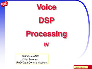
VoiceDSPProcessingIV Yaakov J. Stein Chief ScientistRAD Data Communications
Voice DSP Part 1 Speech biology and what we can learn from it Part 2 Speech DSP (AGC, VAD, features, echo cancellation) Part 3 Speech compression techiques Part 4 Speech Recognition
Voice DSP - Part 4 Speech Recognition tasks ASR Engine Pattern Recognition and Phonetic labeling DTW HMM State-of-the-Art
Speech Recognition Tasks • ASR - Automatic Speech Recognition (speech-to-text) • Language/Accent Identification • Keyword-spotting/Gisting/Task-related • Isolated-word/Connected-word/Continuous-speech • Speaker-dependent/Speaker-adaptive/Speaker-independent • Small-vocabulary/Large-vocabulary/Arbitrary-input • Constrained-grammar/Free-speech • Speaker Recognition • Gender-only • Text-dependent/Text-independent • Speaker-spotting/Speaker-verification/Forensic • Closed-set/open-set • Misc • Emotional-state/Voice-polygraph • Translating-telephone • Singing
Basic ASR Engine Acoustic Processing Phonetic Labeling Time Alignment speech Dictionary & Syntactic Processing Semantic Processing text Notes: not all elements are present in all systems we will not discuss syntactic/semantic processing here
Acoustic Processing … All the processing we have learned before • AGC • VAD • Filtering • Echo/noise cancellation • Pre-emphasis • Mel/Bark scale spectral analysis • Filter banks • LPC • Cepstrum ...
Phonetic labeling • Some ASR systems attempt to label phonemes • Others don’t label at all, or label other pseudo-acoustic entities • Labeling simplifies overall engine architecture • Changing speaker/language/etc. has less system impact • Later stages are DSP-free
Phonetic Labeling - cont. Peterson - Barney data - an attempt at labeling in formant space
Phonetic Labeling - cont. Phonetic labeling is a classical Pattern Recognition task independence of Need channel, speaker, speed, etc adaptation to Pattern recognition can be computationally complex so feature extraction is often performed for data dimensionality reduction (but always loses information) Commonly used features: • LPC • LPC cepstrum (shown to be optimal in some sense) • (mel/Bark scale) filter-bank representation • RASTA (good for cross-channel applications) • Cochlea model features (high dimensionality)
Pattern Recognition Quick Review What is Pattern Recognition ? • classification of real-world objects Not a unified field(more ART than SCIENCE) Not trivial (or even well-defined) 1, 2, 3, 4, 5, 6, 7, and the answer is ... 1, 2, 3, 4, 5, 6, 7, 5048 because I meant [n + (n-1)(n-2)(n-3)(n-4)(n-5)(n-6)(n-7) ]
Pattern Recognition - approaches Approaches to Pattern Recognition • Statistical (Decision Theoretic) • Syntactical (Linguistic) Syntactical Method • Describe classes by rules (grammar) in a formal language • Identify pattern's class by grammar it obeys • Reduces classification to string parsing • Applications: Fingerprinting, Scene analysis, Chinese OCR Statistical Method (here concentrate on this) • Describe patterns as points in n dimensional vector space • Describe classes as hypervolumes or statistical clouds • Reduces classification to geometry or function evaluation • Applications: Signal classification, Speech, Latin OCR
PR Approaches - examples Class A Class B Class C Statistical ( 1, 0, 0 ) ( 0, 1, 0 ) ( 0, 0, 1 ) (0.9, 0.1, 0) (0.1, 1, -0.1) (-0.1, 0.1, 1) (1.1, 0, 0.1) (0, 0.9, -0.1) (0.1, 0, 1.1) Syntactic ( 1, 1, 1 ) ( 1, 2, 3 ) ( 1, 2, 4 ) ( 2, 2, 2 ) ( 2, 3, 4 ) ( 2, 4, 8 ) ( 3, 3, 3 ) ( 3, 4, 5 ) ( 3, 6, 12)
Classifier types Decision theoretic pattern recognizers come in three types: Direct probability estimation 1NN, kNN, Parzen, LBG, LVQ Hypersphere potentials, Mahalanobis (MAP for Gauss), RBF, RCE Hyperplane Karhunen-Loeve, Fisher discriminant, Gaussian mixture classifiers, CART, MLP
Learning Theory Decision theoretic pattern recognizer is usually trained Training (learning) algorithms come in three types • Supervised (learning by examples, query learning) • Reinforcement (good-dog/bad-dog, TDl) • Unsupervised (clustering, VQ) Cross Validation: In order not to fall into the generalization trap we need • training set • validation set • test set (untainted, fair estimate of generalization) Probably Approximately Correct Learning • teacher and student • VC dimension - strength of classifier • Limit on generalization error Egen - Etr < a dVC/ Ntr
Why ASR is not pattern recognition Say pneumonoultramicroscopicsilicovolcanoconiosis I bet you can’t say it again! pneumonoultramicroscopicsilicovolcanoconiosis • I mean pronounce precisely the same thing • It might sound the same to your ear (+ brain), • but the timing will never be exactly the same • The relationship is one of nonlinear time warping
Time Warping The Real Problem in ASR - we have to correct for the time warping Note that since the distortion is time-variant it is not a filter! One way to deal with such warping is to use Dynamic Programming The main DP algorithm has many names • Viterbi algorithm • Levenshtein distance • DTW but they are all basically the same thing! The algorithm(s) are computationally efficient since they find a global minimum based on local decisions
Levenshtein Distance Easy case to demonstrate - distance between two strings Useful in spelling checkers, OCR/ASR post-processors, etc There are three possible errors • Deletion digital - digtal • Insertion signal - signall • Substitution processing - prosessing The Levenshtein distance is the minimal number of errors distance between dijitl and digital is 2 How do we find the minimal number of errors? Algorithm is best understood graphically
Levenshtein distance - cont. Rules: 1enter square from left (deletion) cost = 1 2enter square from under (insertion) 3aenter square from diagonal and same letter cost = 0 3benter square from diagonal and different letter (substitution) cost = 1 4 Always use minimal cost What is the Levenshtein distance between prossesing and processing? p r o s s e s i n g p r o c e s s i n g
Levenshtein distance - cont. Start with 0 in the bottom left corner 9 8 7 6 5 4 3 2 1 0 1 2 3 4 5 6 7 8 9 p r o s s e sin g p r o c e s s i n g 0
p r o s s e sin g p r o c e s s i n g Levenshtein distance - cont. Continue filling in table 9 8 7 6 5 4 3 2 2 2 3 2 1 1 2 2 1 0 1 2 1 0 1 2 3 0 1 2 3 4 5 6 7 8 9 Note that only local computations and decisions are made 0
p r o s s e sin g p r o c e s s i n g Levenshtein distance - cont. Finish filling in table 9 8 7 7 6 5 5 5 4 3 8 7 6 6 5 4 4 4 3 4 7 6 5 5 4 3 3 3 5 5 6 5 4 4 3 2 3 4 4 5 5 4 3 3 2 3 3 3 4 5 4 3 2 2 2 2 2 3 4 5 3 2 1 1 2 2 3 4 5 6 2 1 0 1 2 3 4 5 6 7 1 0 1 2 3 4 5 6 7 8 0 1 2 3 4 5 6 7 8 9 The global result is 3 ! 0
p r o s s e sin g p r o c e s s i n g Levenshtein distance - end Backtrack to find path actually taken 9 8 7 7 6 5 5 5 4 3 8 7 6 6 5 4 4 4 3 4 7 6 5 5 4 3 3 3 4 5 6 5 4 4 3 23 4 4 5 5 4 3 3 2 3 3 3 4 5 4 3 2 222 2 3 4 5 3 2 1 12 2 3 4 5 6 2 1 0 1 2 3 4 5 6 7 1 0 1 2 3 4 5 6 7 8 0 1 2 3 4 5 6 7 8 9 Remember: The question is always how we got to a square
Generalization to DP What if not all substitutions are equally probable? Then we add a cost function instead of 1 We can also have costs for insertions and deletions Di j = min ( Di-1 j + Ci-1 j; I j ; Di-1 j-1 + Ci-1 j-1; I j ; Di j-1 + Ci-1 j; I j ) Even more general rules are often used
DTW DTW uses the same technique for matching spoken words The input is separately matched to each dictionary word and the word with the least distortion is the winner! When waveforms are used the comparison measure is: correlation, segmental SNR, Itakura-Saito, etc When (N) features are used the comparison is (N-dimensional) Euclidean distance With DTW there is no labeling, alignment and dictionary are performed together
DTW - cont. Some more details: In isolated word recognition systems energy contours are used to cut the words linear time warping is then used to normalize the utterance special mechanisms are used for endpoint location flexibility so there are endpoint and path constraints In connected word recognition systems the endpoint of each recognized utterance is used as a starting point for searching for the next word In speaker-independent recognition systems we need multiple templates for each reference word the number of templates can be reduced by VQ
a11 a44 a33 a22 probabilities a12 a34 a23 a11 a44 a33 a22 a12 a23 a34 a13 a24 Markov Models An alternative to DTW is based on Markov Models A discrete-time left-to-right first order Markov model A DT LR second order Markov model a12 a11 + a12 = 1, a22 + a23 = 1, etc. State 1 2 3 4 a11 + a12 + a13 = 1, a22 + a23 + a24 = 1, etc.
3 1 2 4 Markov Models - cont. General DT Markov Model Model jumps from state to state with given probabilities e.g. 1 1 1 1 2 2 3 3 3 3 3 3 3 3 4 4 4 or 1 1 2 2 2 2 2 2 2 2 2 4 4 4 (LR models)
Markov Models - cont. Why use Markov models for speech recognition? • States can represent phonemes (or whatever) • Different phoneme durations (but exponentially decaying) • Phoneme deletions using 2nd or higher order So time warping is automatic ! We build a Markov model for each word given an utterance, select the most probable word
HMM But the same phoneme can be said in different ways so we need a Hidden Markov Model a11 a44 a33 a22 a12 a34 a23 b14 b11 b13 b12 4 1 3 2 aij are transition probabilities bik are observation (output) probabilities acoustic phenomenon b11 + b12 + b13 + b14 = 1, b21 + b22 + b23 + b24 = 1, etc.
HMM - cont. For a given state sequence S1 S2 S3 … ST the probability of an observation sequence O1 O2 O3 … OT is P(O|S) =bS1O1 bS2O2 bS3O3 …bSTOT For a given hidden Markov model M = { p,a, b } the probability of the state sequence S1 S2 S3 … ST is (the initial probability ofS1 is taken to bepS1) P(S|M) =pS1aS1S2aS2S3aS3S4…aST-1ST So, for a given hidden Markov model M the probability of an observation sequence O1 O2 O3 … OT is obtained by summing over all possible state sequences
HMM - cont. P(O| M) = S P(O|S) P(S|M) = SpS1bS1O1 aS1S2bS2O2 aS2S3bS2O2 … So for an observation sequence we can find the probability of any word model (but this can be made more efficient using the forward-backward algorithm) How do we train HMM models? The full algorithm (Baum-Welch) is an EM algorithm An approximate algorithm is based on the Viterbi (DP) algorithm (Sorry, but beyond our scope here)
State-of-the-Art Isolated digits Isolated words Constrained Free speech Spkr dep@100% 98% 95% 90% Spkr ind> 98% 95% 85% < 70% NB 95% on words is about 50% on sentences only > 97% is considered useful for transcription (otherwise more time consuming to correct than to type)