Download
1 / 60
600 likes | 908 Vues
International Economics 2. Economic Growth in Open Economies. International Economics. 2. Economic Growth in Open Economies 2.1. The Balance of Payments 2.2. The Solow-Swan Model 2.3. Economic Policy Conclusions 2.4. Questions for Review Additional Literature :

E N D
International Economics2. Economic Growth in Open Economies Prof. Dr. Rainer Maurer
International Economics 2. Economic Growth in Open Economies 2.1. The Balance of Payments 2.2. The Solow-Swan Model 2.3. Economic Policy Conclusions 2.4. Questions for Review Additional Literature: ◆ Kapitel 15, Siebert, Horst; Einführung in die Volkswirtschaftslehre; Kohlhammer. ◆ Kapitel 27, Abschnitt 9, Baßler, Ulrich, et al.; Grundlagen und Probleme der Volkswirtschaft, Schäfer-Pöschel. Prof. Dr. Rainer Maurer
International Economics 2. Economic Growth in Open Economies 2.1. The Balance of Payments Prof. Dr. Rainer Maurer
2. Economic Growth in Open Economies2.1. The Balance of Payments • The balance of payments records the relationship between a country's merchandise trade and the capital movements of a country with foreign countries. • The relationship between merchandise trade and capital movements follows from the double-entry bookkeeping system of national accounting. • It is an accounting identity, which means, it always valid - if all transactions with foreign countries are properly recorded by this bookkeeping system. • According to neoclassical growth theory (= Solow-Swan model), this relationship represents the direct influence of foreign countries on domestic GDP growth. Prof. Dr. Rainer Maurer
2. Economic Growth in Open Economies2.1. The Balance of Payments • It is easy to derive the balance of payments of a country from the expenditure account of GDP (cf. Macroeconomics AU 1.3.2) and the government budget constraint. • Expenditure account of GDP : GDP (=Y) = Consumption of Housholds (= C) + Net investment (= I) + Capital depreciation (= λ*K) + Government consumption (= G) + Exports (= X) ./. Imports (= M) • Government budget constraint : Government consumption (=G) = Tax payments (=T) + New indebtedness (=DG) Prof. Dr. Rainer Maurer
Expenditure account of GDP : BIP = C + I + λ * K + G + X – M <=> BIP – C – I - λ * K – G = X – M | G = T + DG <=> BIP – C – I - λ * K – (T + DG )= X – M <=> BIP - λ * K – T – C – (I + DG )= X – M <=> S – (I + DG )= X – M 2. Economic Growth in Open Economies2.1. The Balance of Payments Prof. Dr. Rainer Maurer
2. Economic Growth in Open Economies2.1. The Balance of Payments S – (I + DG )= X – M Foreign demand for domestic goods Domestic Savings Domestic demand for foreign goods Domestic Capital Demand = Balance of capital payments Balance of current account1) 1)Strictly speaking is EX-IM only equal to the so called „Net exports“ (Domestic concept). In order to achieve the complete balance of capital and current account (national concept), the balance of income with foreign countries as well as the balance of the transfers between nationals and foreigners must be added. The exact current account balance is obtained if the above calculation steps are carried out not with the GDP but with the Gross National Product (GNP). For the sake of simplicity, these subtleties are neglected. Prof. Dr. Rainer Maurer
2. Economic Growth in Open Economies2.1. The Balance of Payments The settlement of the balance of payments (i.e. balance of payments balance = 0) is a mathematical necessity (tautology), which follows (as seen above) from the expenditure account of GDP. Balance of capital payments = Balance of current account Balance of capital payments - Balance of current account = 0 = 0 Balance of payments Prof. Dr. Rainer Maurer
2. Economic Growth in Open Economies2.1. The Balance of Payments St – (It + DG,t)= Xt – Mt >0 Net credit supply to foreign countries >0 Net exports to foreign countries = If exports are larger than imports (=positive balance of current account = current account surplus), credit supply to foreign countries must also be larger than credit supply from foreign countries (=positive balance of capital payments). => Foreign countries will run into debt, if the current account balance is positive! Prof. Dr. Rainer Maurer
2,1% 17% 17,2% 28,5% Prof. Dr. Rainer Maurer
2. Economic Growth in Open Economies2.1. The Balance of Payments St – (It + DG,t)= Xt – Mt <0 Net credit supply to foreign countries <0 Net exports to foreign countries = If imports are larger than exports (=negative balance of current account = current account deficit), credit supply to foreign countries must be smaller than credit supply from foreign countries (=negative balance of capital payments). => The home country will run into debt, if the current account balance is negative! Prof. Dr. Rainer Maurer
2. Economic Growth in Open Economies2.1. The Balance of Payments => Net foreign asset position = accumulated capital- resp. current account balances: Net foreign asset position • Important: Due to changes of the Euro denominated market values of assets, deviations from this formula are possible. • Countries, which typically have positive current account balances, have a growing positive net foreign asset position, i.e. they are accumulating net wealth. • Countries, which typically have negative current account balances, have a growing negative net foreign asset position, i.e. they run into debt. Prof. Dr. Rainer Maurer
2. Economic Growth in Open Economies2.1. The Balance of Payments The historical development of the current account deficit of the US shows that even long-term current account deficits (over 70 years!) can be sustainableif the debts granted from abroad are not used for consumption but are used for investments. From 1820 to 1890, the United States built up infrastructure (railways, bridges, channels, port facilities) and industrial production facilities with the help of foreign capital flowing from Europe to the US via the London financial market. When these investments yielded a return, the US were able to repay their debts. By the year 1910, the net asset position of the US became positive. If the US had used the foreign loans for consumption, a repayment would not have been possible. Prof. Dr. Rainer Maurer
Phase 1: Infrastrucure investment (railways, bridges, chanels, ports), Buildup of real capital stock Phase 2: Trade balance surplus < interest payment Phase 3: Trade balance surplus > interest payment Prof. Dr. Rainer Maurer Source: Sachs/Larrain (1993)
Phase 4: Net creditor Phase 5: Start of the 70s: Financing of trade balance deficits with interest surpluses Phase 6: End of 70s: Current account deficits Source: Sachs/Larrain (1993) Phase 7: Net debtor because of government debt and high-tech investment boom Prof. Dr. Rainer Maurer
International Economics 2. Economic Growth in Open Economies 2.1. The Balance of Payments 2.2. The Solow-Swan Model Prof. Dr. Rainer Maurer
2. Economic Growth in Open Economies2.2. The Solow-Swan Model • In the lecture “Macroeconomics” the neo-classical growth theory was discussed for the case of a closed economy (= Autarky), to simplify the analysis. • This implies that a country has no economic relations with foreign countries: Exports and Imports are equal to zero. => St – It = Ext – Imt = 0 => St = It • In this case, savers can only invest their savings in the domestic economy. • The interest rate thus ensures that the savings curve S(Y) always equals the investment curve I(i). • We will repeat this in the following (Macroeconomics chapter 2, slides 25 -35) before we go on with the case of an open economy. Prof. Dr. Rainer Maurer
2. Economic Growth in Open Economies2.2. The Solow-Swan Model Y Y(A,B,P,L,H,K) K * λ S = s*Y= I K * λ = Depreciation of the capital stock 5 => λ = 5/7 = 71% = Depreciation rate K Prof. Dr. Rainer Maurer 7
2. Economic Growth in Open Economies2.2. The Solow-Swan Model Up to what point does the GDP of this economy grow when the capital stock has reached at Kt? Y Y(A,B,P,L,H,K) K * λ S = s*Y= I K Kt Prof. Dr. Rainer Maurer
2. Economic Growth in Open Economies2.2. The Solow-Swan Model Y Y(A,B,P,L,H,K) K*λ Yt S = s*Y= I Ct St = It K Kt Prof. Dr. Rainer Maurer
2. Economic Growth in Open Economies2.2. The Solow-Swan Model Y Y(A,B,P,L,H,K) K*λ Yt S = s*Y= I Ct = ΔKt+1= Kt+1 – Kt Kt * λ K Kt Prof. Dr. Rainer Maurer
2. Economic Growth in Open Economies2.2. The Solow-Swan Model Y Y(A,B,P,L,H,K) K*λ Yt S = s*Y= I Ct = ΔKt+1= Kt+1 - Kt Kt * λ K Prof. Dr. Rainer Maurer Kt ΔKt+1 Kt+1
2. Economic Growth in Open Economies2.2. The Solow-Swan Model Y Y(A,B,P,L,H,K) K*λ Yt+1 Ct+1 Yt S = s*Y= I = ΔKt+2= Kt+2 – Kt+1 Kt+1 * λ K Prof. Dr. Rainer Maurer Kt Kt+1 Kt+2 ΔKt+2
2. Economic Growth in Open Economies2.2. The Solow-Swan Model Y Y(A,B,P,L,H,K) Yt+2 K*λ Yt+1 Ct+2 Yt S = s*Y= I = ΔKt+3= Kt+3 – Kt+2 Kt+2 * λ K Prof. Dr. Rainer Maurer Kt Kt+2 Kt+1 Kt+3 ΔKt+3
4. Die langfristige Entwicklung von Volkswirtschaften 4.1. Das Solow-Swan Modell einer geschlossenen Volkswirtschaft Y Y(A,B,P,L,H,K) Yt+3 Yt+2 K*λ Yt+1 Ct+3 Yt S = s*Y= I = ΔKt+4= Kt+4 – Kt+3 Kt+3 * λ K Prof. Dr. Rainer Maurer Kt Kt+2 Kt+3 Kt+1 ΔKt+4 Kt+4
2. Economic Growth in Open Economies2.2. The Solow-Swan Model Y Y(A,B,P,L,H,K) Y*t Yt+4 Yt+3 Yt+2 K*λ Yt+1 C*t Yt s*Y(A,B,P,L,H,K)= I Kt+1 – Kt = 0 I*t = Kt * λ Steady State! K K*t Prof. Dr. Rainer Maurer Kt+2 Kt+3 Kt+4 Kt+1
2. Economic Growth in Open Economies2.2. The Solow-Swan Model • In an open economy, this adjustment process changes: • Domestic savers have then the possibility to invest their money in the country with the highest interest rate. • Domestic investment has no longer necessarily to equal domestic savings. • As seen in section 2.1. the following is now possible: Prof. Dr. Rainer Maurer
Capital Market in a Small Open Economy Case of aclosedeconomy (Autarky) i S = s*Y Since domestic savings can not flow abroad, the domestic interest rate adjusts in such a way that domestic investment demand is always just as large as domestic savings. iWorld market Dom. savings iAutarky Dom. investment I(i,K,A,P,L,H,B) I, S Prof. Dr. Rainer Maurer
Capital Market in a Small Open Economy Case of anopeneconomy i S = s*Y Dom. Savings iWorld market Dom. Investment Capital export (=KX) in an open economy if the world interest rate is higher than the domestic autarky interest rate. iAutarky I(i,K,A,P,L,H,B) Locals invest their savings in foreign countries. => Domestic investment falls compared to autarky! I, S I < S Prof. Dr. Rainer Maurer
Capital Market in a Small Open Economy Case of anopeneconomy i S = s*Y Foreigners invest their money in the domestic economy. => Domestic investment grows compared to autarky! Capital imports (=KM) in an open economy if the domestic autarky interest rate is higher than the world market interest rate . iAutarky Dom. Savings iWorld market I(i,K,A,P,L,H,B) Dom. Investment I, S S < I Prof. Dr. Rainer Maurer
2. Economic Growth in Open Economies2.2. The Solow-Swan Model • This means: • If the world market interest rate is lower than the domesticmarket interest rate in case of autarky, • the inland borrows from foreign countries and • purchases with these credits goods in foreign countries, • which are then invested in the domestic capital stock. => The domestic capital stock does then grow faster as in the case of autarky and its steady state level is higher. Capital import (KMt = St -It < 0 ) comesalongwith a currentaccountdeficit: St – It = Xt – Mt< 0 Prof. Dr. Rainer Maurer
2. Economic Growth in Open Economies2.2. The Solow-Swan Model Y Capital import Y(A,B,P,L,H,K) K * λ Y*1 I= s*Y + KM S = s*Y Capital import (=KM) in an open economy, if the autarky interest rate is higher than the world market interest rate. K K*1 Prof. Dr. Rainer Maurer
2. Economic Growth in Open Economies2.2. The Solow-Swan Model Y Capital import Y(A,B,P,L,H,K) Y*2 K * λ Y*1 I= s*Y + KM S = s*Y Due to capital imports, the steady state capital stock is higher as under autarky! K K*2 K*1 Prof. Dr. Rainer Maurer
2. Economic Growth in Open Economies2.2. The Solow-Swan Model • Thus steady state GDP is higher because of capital imports. • However, interest to foreigners has to be paid for the credits received from foreigner: • As a result, a part of the income generated domestically flows as interest payments abroad every year. • Gross National Product (GNP = the part of income, which flows to residents) in case of capital import is smaller than GDP. • A mathematical calculation of the impact of capital imports on domestic incomes shows that the net effect is typically positive : • Not only interest payments are sent abroad, but the immobile domestic production factors (especially the labor) also receive higher remuneration because the higher steady state capital stock increases their productivity. Prof. Dr. Rainer Maurer
2. Economic Growth in Open Economies2.2. The Solow-Swan Model Y Capital import Y(A,B,P,L,H,K) Y*2 GNP2 K * λ Y*1 I= s*Y + KM Interest payments to foreign savers S = s*Y Part of the higher GDP flows in the form of interest payments to foreign countries. As a result, in case of capital imports, the incomes of the residents grow somewhat less than the GDP. K K*2 K*1 Prof. Dr. Rainer Maurer
2. Economic Growth in Open Economies2.2. The Solow-Swan Model • In the obverse case: • If the world market interest rate is higher than the domesticmarket interest rate in case of autarky, • the foreign countries borrow from the inland and • purchase with these credits goods from the inland, • which are then invested inforeign capital stocks. => The domestic capital stock does then grow slower as in the case of autarky and its steady state level is lower. Capital export (KXt= St - It> 0 ) comesalongwith a currentaccountsurplus: St – It = Xt – Mt> 0 Prof. Dr. Rainer Maurer
Capital Market in a Small Open Economy Case of anopeneconomy i S = s*Y Dom. Savings iWorld market Dom. Investment Capital export (=KX) in an open economy if the world interest rate is higher than the domestic autarky interest rate. iAutarky I(i,K,A,P,L,H,B) Locals invest their savings in foreign countries. => Domestic investment falls compared to autarky! I, S I < S Prof. Dr. Rainer Maurer
2. Economic Growth in Open Economies2.2. The Solow-Swan Model Capital export Y Y(A,B,P,L,H,K) K * λ Y*1 S = s*Y I= s*Y - KX Capital export (=KX) in an open economy, if the autarky interest rate is higher than the world market interest rate. K K*1 Prof. Dr. Rainer Maurer
2. Economic Growth in Open Economies2.2. The Solow-Swan Model Capital export Y Y(A,B,P,L,H,K) K * λ Y*1 Y*2 S = s*Y I= s*Y - KX Caused by capital exports the resulting steady state capital stock is lower! K K*2 K*1 Prof. Dr. Rainer Maurer
2. Economic Growth in Open Economies2.2. The Solow-Swan Model • Thus steady state GDP is lower because of capital exports. • However, interest to domestic savers has to be paid for the credits received from them: • As a result, a part of the income generated abroad flows as interest payments to domestic savers every year. • Gross National Product (GNP = the part of income, which flows to residents) in case of capital import is higher than GDP. • A mathematical calculation of the impact of capital imports on domestic incomes shows that the net effect is, however, typically negative: • Despite of the interest payments from abroad, the immobile domestic production factors (especially the labor) also receive a lower remuneration because the smaller steady state capital stock decreases their productivity. Prof. Dr. Rainer Maurer
2. Economic Growth in Open Economies2.2. The Solow-Swan Model Capital export Y Y(A,B,P,L,H,K) Y*1 K * λ GNP2 Y*2 S = s*Y Interest payments to foreign savers I= s*Y - KX Part of the foreign GDP flows in the form of interest payments to the domestic economy. Therefore, the incomes of the residents decrease somewhat less than GDP. K K*2 K*1 Prof. Dr. Rainer Maurer
2. Economic Growth in Open Economies2.2. The Solow-Swan Model • Conclusions: • In order to keep a "high" domestic capital stock (and thus a high GDP) in the case of free international capital movements, savers must be able to receive a high interest rate for their money in the domestic economy. • Thus, there must be sufficient investment opportunities with a high yield in the domestic economy. • Only in this case, the domestic demand for credits is high enough. This is displayed by the domestic investment demand curve in next chart. • The domestic investment demand curve must therefore lie on a "high" level. Prof. Dr. Rainer Maurer
Capital Market in a Small Open Economy i S = s*Y iWorld market iAutarky I(i,K1,A1,P1,L1,H1B1) Domestic investment demand curve I, S I = S Prof. Dr. Rainer Maurer
Capital Market in a Small Open Economy i Capital import (=KM) in an open economy, if the autarky interest rate is higher than the world market interest rate. . S = s*Y iAutarky,2 Dom. Savings iWorld market iAutarky,1 I(i,K1,A2,P2,L2,H2,B2) Domestic Investment I(i,K1,A1,P1,L1,H1,B1) A1<A2, P1<P2, L1<L2, H1<H2, B1<B2 I, S I = S Prof. Dr. Rainer Maurer
2. Economic Growth in Open Economies2.2. The Solow-Swan Model • Conclusion: • When lessinvestment opportunities with high returns are available in the domestic economy, savers place their money abroad, where they receive higher returns. • In this case, the domestic investment demand curve shifts downward. • The result is then capital export, as the next chart shows. Prof. Dr. Rainer Maurer
Capital Market in a Small Open Economy i S = s*Y Capital export (=KX) in an open economy, if the autarky interest rate is lower than the world market interest rate. Domestic investment iAutarky,1 iWorld market iAutarky,2 Dom. Savings I(i,K1,A1,P1,L1,H1,B1) I(i,K1,A2,P2,L2,H2,B2) A1>A2, P1>P2, L1>L2, H1>H2, B1>B2 I, S I = S Prof. Dr. Rainer Maurer
International Economics 2. Economic Growth in Open Economies 2.1. The Balance of Payments 2.2. The Solow-Swan Model 2.3. Economic Policy Conclusions Prof. Dr. Rainer Maurer
2. Economic Growth in Open Economies2.3. EconomicPolicyConclusions • This leads to the question, how a country can provide investment opportunities with a high return, i.e. how to keep the domestic investment demand curve on a “high” level? • The answer of standard production theory is: • A country must try to accumulate as many production factors as possible, which are complementary to capital. • Production factors, which are complementary to capital, increase the productivity of the capital stock and thus lead to a higher return on capital investments. • As a result, the domestic investment demand grows and the investment demand curve lies at a higher level. Prof. Dr. Rainer Maurer