Download
1 / 1
10 likes | 152 Vues
Understanding Quasar Variability through Kepler Dan Silano 1 , Paul J. Wiita 1 , Ann E. Wehrle 2 , and Stephen C. Unwin 3 1 The College of New Jersey, Department of Physics, P.O. Box 7718, Ewing, NJ 08628, wiitap@tcnj.edu, silano2@tcnj.edu

E N D
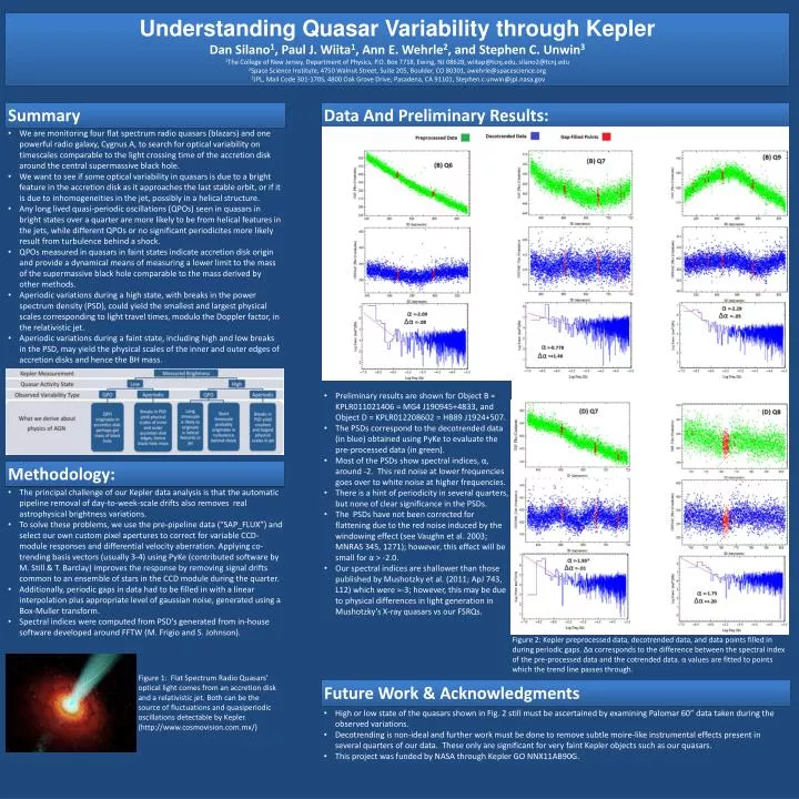
Understanding Quasar Variability through Kepler Dan Silano1, Paul J. Wiita1, Ann E. Wehrle2, and Stephen C. Unwin3 1The College of New Jersey, Department of Physics, P.O. Box 7718, Ewing, NJ 08628, wiitap@tcnj.edu, silano2@tcnj.edu 2Space Science Institute, 4750 Walnut Street, Suite 205, Boulder, CO 80301, awehrle@spacescience.org 3JPL, Mail Code 301-170S, 4800 Oak Grove Drive, Pasadena, CA 91101, Stephen.c.unwin@jpl.nasa.gov Data And Preliminary Results: Summary • We are monitoring four flat spectrum radio quasars (blazars) and one powerful radio galaxy, Cygnus A, to search for optical variability on timescales comparable to the light crossing time of the accretion disk around the central supermassive black hole. • We want to see if some optical variability in quasars is due to a bright feature in the accretion disk as it approaches the last stable orbit, or if it is due to inhomogeneities in the jet, possibly in a helical structure. • Any long lived quasi-periodic oscillations (QPOs) seen in quasars in bright states over a quarter are more likely to be from helical features in the jets, while different QPOs or no significant periodicites more likely result from turbulence behind a shock. • QPOsmeasured in quasars in faint states indicate accretion disk origin and provide a dynamical means of measuring a lower limit to the mass of the supermassive black hole comparable to the mass derived by other methods. • Aperiodic variations during a high state, with breaks in the power spectrum density (PSD), could yield the smallest and largest physical scales corresponding to light travel times, modulo the Doppler factor, in the relativistic jet. • Aperiodic variations during a faint state, including high and low breaks in the PSD, may yield the physical scales of the inner and outer edges of accretion disks and hence the BH mass. • Preliminary results are shown for Object B = KPLR011021406 = MG4 J190945+4833, and Object D = KPLR012208602 = HB89 J1924+507. • The PSDs correspond to the decotrended data (in blue) obtained using PyKe to evaluate the pre-processed data (in green). • Most of the PSDs show spectral indices, α, around -2. This red noise at lower frequencies goes over to white noise at higher frequencies. • There is a hint of periodicity in several quarters, but none of clear significance in the PSDs. • The PSDs have not been corrected for flattening due to the red noise induced by the windowing effect (see Vaughn et al. 2003; MNRAS 345, 1271); however, this effect will be small forα > -2.0. • Our spectral indices are shallower than those published by Mushotzky et al. (2011; ApJ 743, L12) which were ≈-3; however, this may be due to physical differences in light generation in Mushotzky’s X-ray quasars vs our FSRQs. Methodology: • The principal challenge of our Kepler data analysis is that the automatic pipeline removal of day-to-week-scale drifts also removes real astrophysical brightness variations. • To solve these problems, we use the pre-pipeline data (“SAP_FLUX”) and select our own custom pixel apertures to correct for variable CCD-module responses and differential velocity aberration. Applying co-trending basis vectors (usually 3-4) using PyKe (contributed software by M. Still & T. Barclay) improves the response by removing signal drifts common to an ensemble of stars in the CCD module during the quarter. • Additionally, periodic gaps in data had to be filled in with a linear interpolation plus appropriate level of gaussian noise, generated using a Box-Muller transform. • Spectral indices were computed from PSD's generated from in-house software developed around FFTW (M. Frigio and S. Johnson). Figure 2: Kepler preprocessed data, decotrended data, and data points filled in during periodic gaps. Δα corresponds to the difference between the spectral index of the pre-processed data and the cotrended data. α values are fitted to points which the trend line passes through. Figure 1: Flat Spectrum Radio Quasars’ optical light comes from an accretion disk and a relativistic jet. Both can be the source of fluctuations and quasiperiodic oscillations detectable by Kepler. (http://www.cosmovision.com.mx/) Future Work & Acknowledgments • High or low state of the quasars shown in Fig. 2 still must be ascertained by examining Palomar 60” data taken during the observed variations. • Decotrending is non-ideal and further work must be done to remove subtle moire-like instrumental effects present in several quarters of our data. These only are significant for very faint Kepler objects such as our quasars. • This project was funded by NASA through Kepler GO NNX11AB90G.