Download
1 / 41
410 likes | 533 Vues
Global seismic tomography and its CIDER applications. Adam M. Dziewon ski. KITP, July 14, 2008. Earth’s boundary layers. Power spectra of three models. Harvard Caltech Berkeley. The properties of a “super-red” spectrum. harmonic order. 15 times more coefficients.

E N D
Global seismic tomography and its CIDER applications Adam M. Dziewonski KITP, July 14, 2008
Power spectra of three models Harvard Caltech Berkeley
The properties ofa “super-red” spectrum harmonic order 15 times more coefficients
Current Issues: • Anisotropy in the lithosphere- asthenosphere system • Transition zone and the fate of the subducted slabs. • Large scale structures in the lower mantle. • Stable layers in the outer core
Velocity Harvard Isotropic shear velocity anomalies at 100 km depth; nearly perfect agreement among different models Berkeley Caltech
Phase velocities in the Pacific Dispersion of Rayleigh waves with 60 second period. Orange is slow, blue is fast. Red lines show the fast axis of anisotropy.
Azimuthal anisotropy under N. America 100 km 200 km 300 km after Marone and Romanowicz, 2007
Observed and predicted SKS splitting measurements after Marone and Romanowicz, 2007
Pacific anisotropy The isotropic variations (top; Voigt average) agree with the pattern of the plate cooling model, even though thermal models predict constant temperature at 150 km depth. The difference between the SV and SH (bottom) velocities at this depth shows no correlation with plate tectonics. from Ekström & Dziewonski, 1998
Pacific cross-section Nettles and Dziewonski, 2008
Radial anisotropy under continents and oceans From Gung et al., 2003
Transition zone boundary layer
Power spectra of the three models;a closer look at the transition zone Harvard Caltech Berkeley angular degree
Harvard Caltech Berkeley 600 km depth 800 km depth
Cross-sections through model TOPO362 from Gu et al., 2003
Change in the stress pattern near the 650 km discontinuity
Izu-Bonin slabStress pattern changes at 500 km depth;is the transition zone full of slabs?
It cannot be this simple; even if it were true, it is not representative of theglobal behavior S-velocity P-velocity Grand et al., 1997
Model S362ANIDepth 750 km l Strong, but spatially limited fast anomalies in the lower mantle may represent regions of limited penetration of subducted material accumulated in the transition zones
Questions: • Why is global topography of the 410 km and 650 km discontinuities de-correlated? • How do the slabs interact with the 650 km discontinuity? • What happens to the slab material after it stagnates in the transition zone? • Why is there such an abrupt change in the spectral power across the 650 km discontinuity?
Power spectra and RMS of models S362ANI and S362D1 After Kustowski et al. (2008)
Power spectra of the three models near the CMB Harvard Caltech Berkeley Kustowski et al. (2008)
2800 km depth from Kustowski, 2006
Equatorial cross-section Dziewonski (1984) and Woodhouse and Dziewonski (1984)
Super-plumes Caltech Scripps
The shape of the African superplume The vertical extent of the two superplumes is much greater than 300 km but velocity anomalies are less than -12% from Wang and Wen (2004)
Generally, models of the shear and compressional velocity are obtained independently. In 1994, Su & Dziewonski obtained P- and S-velocity models by inverting simultaneously a large data set. However, P-velocity depends both on shear modulus and bulk modulus. To isolate this interdependence, Su & Dziewonski (1997) formulated the inverse problem for a joint data set sensitive to P- and S-velocities and derived 3-D perturbations of bulk sound velocity and shear velocity. Trying to understand the super-plumes
Shear and bulk velocity at 550 km ±2% vS ±1% vc Su and Dziewonski, 1997
Shear and bulk velocity at 2800 km vS ±2% ±1% vc Su and Dziewonski, 1997
Bulk Sound and Shear Velocity Anomalies Correlation between the bulk sound and shear velocity anomalies changes from +0.7 in the transition zone to -0.8. From Su and Dziewonski, 1997.
CMB questions: • How have the super-plumes formed? • What part of the anomalies is caused by compositional rather than thermal variations? • Why do the super-plumes continue above the D” without an apparent abrupt change in the amplitude of the anomaly?
Stable layers in the outer core? Generally, the outer core is expected to be well mixed. However, in some 1-D models compressional velocity the gradients at the top and the bottom of the outer core are anomalous, leading to inference that either one or both of these layers are stable.
Core questions • Are there stable layers at the top and bottom of the outer core? • How large is the density contrast between the inner and outer core? • How the properties of the inner core vary with depth? • What is the cause of inner core anisotropy?
Inner-most Inner Core? PKIKP residuals in the distance range from 173 to 180 degrees show anomalous behavior as a function of the ray angle, indicating that anisotropy within 300 - 400 km of the Earth’s center is different from the bulk of the inner core.