Dipole polarizabilities of π ± -mesons

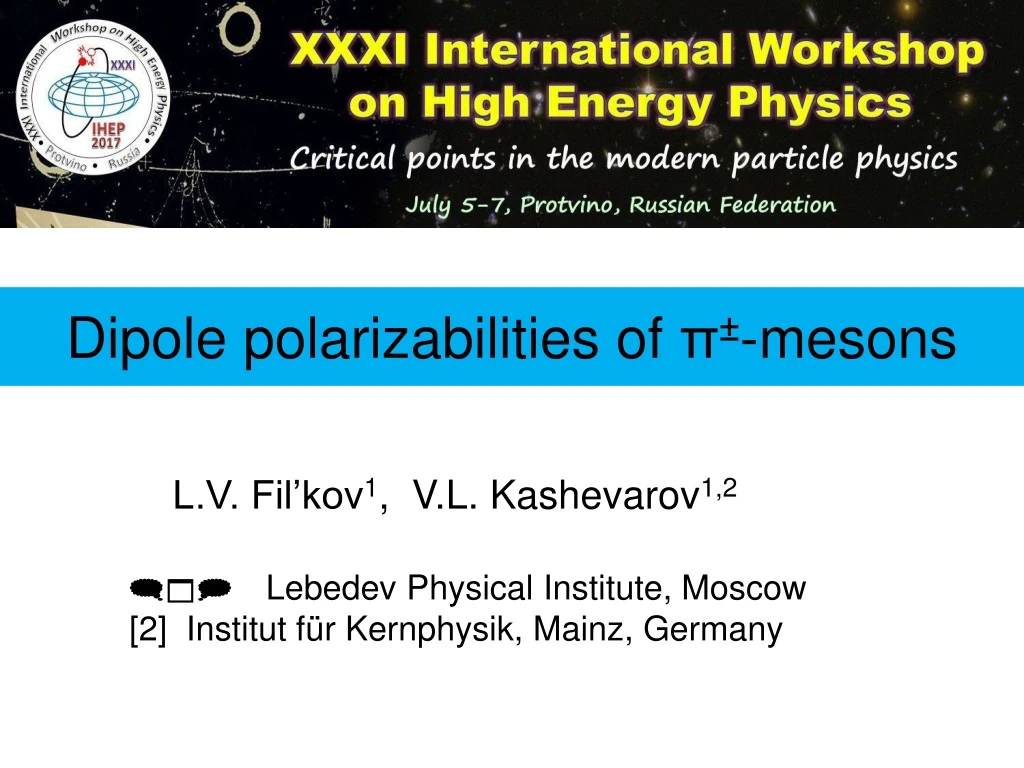
1. Dipole polarizabilities of π±-mesons L.V. Fil’kov1, V.L. Kashevarov1,2 [1] Lebedev Physical Institute, Moscow [2] InstitutfürKernphysik, Mainz, Germany

2. Outline • Introduction. • g + p -> g + p+ +n (Mainz). 3.p-+ Z -> g + p- + Z (Serpukhov). 4. p- + Z -> g + p- + Z (COMPASS). 5.g + g -> p+ + p-. • DSRs and ChPT • Summary

3. The dipole (a1, b1) and quadrupole (a2, b2) pion polarizabilities are defined through the expansion of the non-Born helicity amplitudes of Compton scattering on the pion over t at s=m2 Pion polarizabilities characterize the behavior of the pion in an external electromagnetic field. s=(q1+k1)2, u=(q1–k2)2, t=(k2–k1)2 M++(s=μ2,t)=pm[2(a1 - b1) + t/6 (a2 - b2) + O(t2)] M+-(s=μ2,t)=p/m[2(a1 + b1) + t/6 (a2 + b2) + O(t2)] 15.5x10-4 fm3

4. Review of experimental data on (a1 – b1)p±

5. g + p →g + p+ + n ( MAMI, Eur. Phys. J. A 23, 113 (2005) )

6. where t = (pp –pn )2 = -2mp T, 537 MeV < Eg<817 MeV The cross section of g p→ gp+ n has been calculated in the framework of two different models: • Contribution of all pion and nucleon pole diagrams. • Contribution of pion and nucleon pole diagrams and D(1232), P11(1440), D13(1520), S11(1535) resonances, and σ-meson.

7. To decrease the model dependence we limited ourselves to kinematical regions, where the difference between model-1 and model-2 does not exceed 3% when (α1 – β1)p+ =0. I. The kinematical region where the contribution of (α1 – β1)p+ is small: 1.5 m2 < s1 < 5 m2 Model-1 Model-2 Fit to the experimental data

8. II. The kinematical region where the (α1 – β1)p+ contribution is substantial: 5m2 < s1 < 15m2, -12m2 < t < -2m2 (α1 – β1)p+= (11.6 ± 1.5st ± 3.0sys ± 0.5mod) 10-4 fm3 ChPT (Gasser et al. (2006)): (α1 –β1)p+ = (5.7±1.0) 10-4 fm3

9. p- + Z → p- + g + Z Feff≈ 1 Width of the peak: Maximum of the Coulomb peak at Q2 = 6.8 Serpukhov (Phys. Lett. B 121, 445 (1983) ) Ebeam=40 GeV, 4 ×10-6(GeV/c)2 at w1= 600 MeV Coulomb amplitude dominates for Q2≤ 2 ×10-4(GeV/c)2 Q2 ≤ 6 × 10-4 (GeV/c)2 Q2≈2-8×10-3(GeV/c)2 –estimation of strong background = 13.6 ± 2.8 ± 2.4 Q2 x 103(GeV/c)2

10. p- + Z -> p- + g + ZCOMPASS Collaboration (Phys. Rev. Lett. 114, 062002 (2015)) a1+b1= 0 Ebeam = 190 GeV ( (Serp))/( (COMP)) ≈ 22.5 Q2 ≤ 15 × 10-4 (GeV/c)2 This value of Q2is very far from the Coulomb peak 5×10-4≤Q2≤15×10-4(GeV/c)2 -the interference with the nuclear amplitude is very important. The authors could not describe the bumps in the nuclear cross section at Q>0.04 (GeV/c). At high energies the elastic multiple scattering of hadrons in nuclei is important. (Glauber model) (G.Fäldt, U.Tengblad) Without a real fit to the data it is impossible to estimate the effect of model dependence of the diffractive background. (a1)p±=2.0 ± 0.6 ±0.7

11. Q2 dependence for different Z (Serpukhov) Z2 dependence –an estimation of a contribution of the nuclear background N Q2/GeV2

12. z±= 1 ± cos Qcm Xg=Eg/Ebeam xg 0.4 0.5 0.6 0.7 0.8 0.9 xg Serpukhov COMPASS W ≤ 490 MeV, 0.15 > cosQcm > -1

13. Contribution of the s-meson Contribution of the s-meson z=cosqcm (J.A. Oller, L. Roca – 2008)

14. =4 - COMPASS result (J.A. Oller, L. Roca) Ms= 441 MeV, Gs= 544 MeV, Gsgg= 1.98 keV, gspp= 3.31 GeV, g2sgg = 16pMsGsgg (1) - z= -1 (2) - z= -1 ÷ 0.15 (3)- COMPASS 10 Serpukhov: D(a1-b1)p±≈2.7

15. Total cross section for the reaction g→ p+ p- The cross section is particularly sensitive to at w ≤ 800 MeV. However, the values of the experimental cross section of the process under consideration in this region are very ambiguous. Ms= 441MeV, Gs=544MeV, Gsgg= 1.298keV, g2sgg=16pMsGsgg, gpp=3.31 GeV Result of our fit: (a1-b1)p± = 10 • (a1+b1)p±= 0.107 • (a2-b2)p±=30 • (a2+b2)p±=0.151 280 MeV < w < 500 MeV: Born term, dipole and quadrupole polarizabilities, s-meson

16. DSRs and ChPT • The s-meson is only partialy including in ChPT. • Different methods of vector mesons calculatios in DSRs and ChPT DSR ChPT (Mv/m)2

17. Summary 1.The values of (a1-b1)p±obtained in the Serpukhov, Mainz, and LPI experiments are at variance with the ChPT predictions. 2. In order to improve the result of the Mainz experiment it is necessary to use a better neutron detector and consider other models to fit to the cross section of the process under consideration. 3.The result of the COMPASS Collaboration is in agreement with the ChPT calculations. However, this result is very model dependent. It is necessary to correctly investigate the interference between Coulomb and nuclear amplitudes and take into account the contribution of the s-meson. 4. New, more accurate experimental data on the process gg->p+p-in region W ≤ 800 MeV are needed to obtain reliable values of (a1-b1)p± . 5. Reasons of the discrepancy between the predictions of DSRs and ChPT for (a1-b1)π± are due to the difference in the results of the calculations of the contributions of vector- and s- mesons using these models. 6. It should be noted that the most model independent result was obtained in the Serpukhov experiment.