Download

1 / 26
350 likes | 1.04k Vues
ADSORPTION. 1. Batch adsorption. Rapid adsorption. Mass Balance. On the solute in the liquid. V : tank volume y : effluent concentration y F : fed concentration H : feed rate q : adsorbed concentration. (1). On the adsorbent. (2). r : adsorption rate per tank volume. What r ?.

E N D
1. Batch adsorption Rapid adsorption
Mass Balance • On the solute in the liquid V : tank volume y : effluent concentration yF : fed concentration H : feed rate q : adsorbed concentration (1) • On the adsorbent (2) r : adsorption rate per tank volume
What r ? Mechanisms 1. Adsorption is controlled by diffusion from the solution to the adsorbent. 2. Adsorption is controlled by diffusion and reaction within the adsorbent particles.
Diffusion controls (3) k : mass transfer coefficient a : surface area (adsorbent per tank volume) y*: concentration(equilibrium) (4) Freundlich isotherm
Diffusion and reaction (5) D : diffusion coefficient k : first order irreversible reaction • Adsorption rate-independent of stirring-strong • function of temperature
Solve y(t), q(t) • Combining and integrating 3 or 5 Eqs. 1 and2 + + Equilibrium isotherm
Assume adsorption isotherm as • Integrate equation analytically (6) (7) + : 1 - : 2 (8)
Example 1 Novobiocin Adsorption H : 2.7 liters/hr qo : 1.35g/liter, yF : 640g/cm3, T : 35oC, pH : 6.87.2 Calculate the resin loading q(t). Then estimate the rate constant ka predicted from the simplified theory.
Solution : To find the resin loading, we integrate Eq. (1) : To find k, plot logarithm (yF-y) & time(Fig. 1,next slide) From Eq.6., slop of plot=2(at larger times) From y and q, equilibrium constant K :
Result Eq. 8 Thus
2. FIXED BEDS y(t) : effluent conc. YB : breakthrough conc.(10%) yE : exhaustion conc.(90%) yF l 0
Basic Equations Mass balance in liquid : void fraction in the bed v : superficial velocity(H/A) E : dispersion coefficient (9) Mass balance on the adsorbed solute r : adsorption rate(controlled by mass transfer from bulk solution to the surface of the adsorbent) (10) r : rate per bed volume ka : rate constant y* : concentration in solution at equilibrium (11) Isotherm Equilibrium(adsorbent and solution concentrations) (12)
Nonlinear • Coupled Equations. • Numericallyn solved • For aproximate analysis • - first : breakthrough curves as a ramp • - second : two parameters ( characteristic time, • standard deviation ) • - third : adsorption equilibrium is linear • - fourth : mimic graphical analysis
Depend completely on experiments • 1. Equilibrium zone saturated • 2. Adsorption zone long 2.1 An approximate analysis • Equilibrium zone q(equilibrium)=q(yF) • Adsorption zone contains half of q(yF) as a good approximation • Fraction of the bed which is loaded (A)
2.2 Two parameter model Two parameters : 1. Characteristic time 2. Standard deviation to : time at half feed concentration to : standard deviation(slope of curve)
2.3 Linear adsorption model Linear isotherm (13) Eqs. 9,10,11 and 13 combined Neglects terms : E2/ z2 and y/ t in Eq. 9 and conditions t=0, all z, q=0 t>0, z=0, y=yF
Five parameters : • (y/yF), t, v, K, k - four parameter found - then fifth found
-Moving countercurrently -Infinitely long, steady state -equilibrium, yF and q(yF) -exit solution conc. zero 2.4 Differential contacting model • Mass balance Between the exit and some arbitrary position • Steady state mass balance on the solute in solution accumulation=solute flow(in-out) - solute adsorbed Negligible dispersion Dividing by the volume Az and taking the limit as this volume goes to zero Initial condition Z=0, y=yF
Evaluate - choosing y, integral numericallyand reading q - operating line - using q to find y* from equilibrium
Example 1. Lactate dehydrogenase adsorption L=1.3m, diameter=7cm, void fraction=0.3, feed conc.=1.7mg/liter linear isotherm : q(in mg/cm3)=38y(in mg/cm3) breakthrough 6.4hr, bed exhausted 10hr. (a) the length of the adsorption zone at breakthrough (b) the length of the equilibrium zone at breakthrough (c) the fraction of the bed’s capacity which is being used. Solution a) 10-6.4=3.6hr, so (3.6hr/6.4hr)1.3m=0.73m b) 1.3-0.73=0.57m c) By approximate analysis and from Eq. A =1-(3.6hr/2(6.4hr))=72%
Example 2. Cephalosporin adsorption q(g/liter resin)=32(y(g/liter solution))1/3 bed length : 1.0m, diameter : 3.0, density : 0.67cm3 resin/cm3bed feed conc. : 4.3g/liter, superficial bed velocity : 2m/hr a) Calculate how much of the feed is lost if we stop the adsorption when y=0.4g/liter b) Estimate what fraction of the bed’s capacity is used at this breakthrough. Assume the bed is exhausted when y=4.0g/liter c) Estimate the rate constant in the bed d) If we double the flow rate, how much of the will have been lost when the exit concentration is 0.4g/liter? Solution a) From next slide , breakthrough occurs at 6.3hr thus fraction lost by numerical integration =0.02
b) From the figure, breakthrough = 6.3hr and exhausted = 9.0hr from Eq. (A) c) By linear adsorption model
d) By two parameter model to=7.8hr(inversely proportional to the velocity) =0.15(2 will be directly proportional to the velocity(cf. Table 1)) to : slope of curve y/yF=(0.4/4.0), t=2.4hr lost : about 5%


![protein adsorption [%]](https://cdn3.slideserve.com/5518059/slide1-dt.jpg)