Download

1 / 72
860 likes | 1.75k Vues
Sample Size Estimation. Chulaluk Komoltri DrPH (Bios) Faculty of Medicine Siriraj Hospital. Sample Size Estimation. Why ?. n is large enough to provide a reliable answer to the question too small n a waste of time too many n A waste of money & other resources

E N D
Sample Size Estimation Chulaluk Komoltri DrPH (Bios) Faculty of Medicine Siriraj Hospital
Sample Size Estimation • Why? • n is large enough to provide a reliable answer to the • question • too small n a waste of time • too many n A waste of money & other resources • May be unethical • e.g., delayed beneficial therapy • Study Objective • - Hypothesis generating (Pilot study) • No sample size estimation • - Estimation of parameter, Hypothesis confirmation • Sample size estimation
n is usually determined by the primary objective of the study More than one primary outcomes If one of these endpoints is regarded as more important than others, then calculate n for that primary endpoint. If several outcomes are regarded as equally important, then calculate n for each outcome in turn, and select the largest n. Method of calculating n should be given in the proposal, together with the assumptions made in the calculation
Caution Calculation of sample size needs a number of assumptions and ‘guesstimates’, so such calculation only provides a guideto the number of subjects required.
Pilot study Example: (Mar 23,1999, #1515) This study for n=20 eligible burn patients will generate hypothesis about the predictive values of various patient characteristics for predicting number of days to return to work.
Example: (Oct 27, 1998, #1465) This is a pilot study providing preliminary descriptive statistics thatwill be used to design a larger, adequately powered study. N=24 normal healthy volunteers will be randomized to parallel groups to study the effect of 4 antidepressant drugs…
Estimation study, Hypothesis confirmation study Sample size determination: 2 Objectives I. Estimation of parameter(s) Precision (95% CI) Specify error - Estimate prevalence, sensitivity, specificity - Estimate single mean, single proportion - etc.
II. Test H0 Statistical power (1- ) Specify , error 2.1 Single group - Test of single proportion, mean - Test of Pearson’s correlation - etc. 2.2 Two groups -Test difference of - 2independentproportions, means, survival curves - 2dependent proportions, means - Test equivalence of - 2 independent proportions, means - etc. 2.3 > 2 groups
, (Efficacy trial) Truth H0 true H0 false (A=B) (AB, Difference) Decision Accept H0No error (1- ) (from p-value) (p > ) Reject H0No error (1- ) (p ) Power = Pr (incorrect conclusion of difference ) = False positive (FP) = Pr (incorrect conclusion of equivalence) = False negative (FN) 1 - = Pr ( correct conclusion of difference ) = True positive (TP)
Sample size for estimating parameter, testing hypothesis
nQuery Advisor PASS
1. Estimation 1.1) Estimate single proportion 95% CI of = p ± d where = Pr. of type I error = 0.05 (2-sided) z0.025 = 1.96 p = Estimated proportion of … q = 1-p d = Margin of error in estimating 1.2) Estimate single mean 95% CI of =x ± d n = [z/2 SD / d]2 where SD = Standard deviation of …
95% CI for = p z/2 SE(p) = p z/2 p(1-p)/n = p d Thus, d = z/2 p(1-p) n d2 = z/22 p(1-p) n n = z/22 p(1-p) d2 Derivation of formulas in (1.1), (1.2) 95% CI of = x z/2 SE(x) = x z/2 SD / n = x d Thus, d = z/2 SD n n = z/2 SD 2 d
n = z/22 pq / d2 -----------(1) a) If no idea about p, let p = 0.5 biggest pq = 0.25 At 2-sided = 0.05 then n = 1.962 (0.5)(0.5) 1 -----------(2) d2 d2 b) If finite pop’n (N is known), adjust n from eqn. (1) n = n ------------(3) 1+ n/N = z2pq N ------------(4) d2N + z2pq If n = 1/d2 as in eqn. (2), then n = N ------------(5) (1+d2N)
Conclusion: n = N ---------(5) (1+d2N) where N = Population size d = Margin of error in estimating pop’n proportion Formula # 5 is appropriate under: 1) Objective: To estimate a single proportion 2) Assume p = 0.5 to get the biggest sample size 3) Assume population is finite (known pop’n size N) 4) Assume sample is selected by simple random sampling (SRS)
2)Test 2.1) Test of difference in 2 independent proportions H0 : 1 - 2 = 0 H1 : 1 - 2 0 where = Probability of type I error = Probability of type II error p1 = Proportion of … in gr. 1 q1 = 1-p1 p2 = Proportion of … in gr. 2 q2 = 1-p2 p = (p1+p2)/2 q = 1-p
2.2) Test of difference in 2 independent means H0 : 1 - 2 = 0 H1 : 1 - 2 0 where = Probability of type I error = Probability of type II error = Common standard deviation of … in group 1, 2 = Difference in mean … between 2 groups = 1 - 2
2.3) Test of significance of 1 proportion H0 : = p0 H1 : = p1 where p0 = Proportion of … under H0 p1 = Proportion of … under H1 2.4) Test of significance of 1 mean H0 : = 0 H1 : = 1 where = Standard deviation of … = 1 - 0
2.5) Test of significance of 1 correlation H0 : = 0 H1 : = 1 n = (Z/2 + Z) 2 [F(Z0) - F(Z1)] where F(Z0) = Fisher’s Z transformation of 0 = 0.5 ln [(1+0)/(1-0)] F(Z1) = Fisher’s Z transformation of 1 = 0.5 ln [(1+1)/(1-1)] ln = Natural logarithm + 3
Example 1: (Mar 18, 2000, #1688) This is a cross-sectional study of the prevalence of pulmonary hypertension (PHT) in patients aged 15-70 years with sickle cell disease. The primary endpoint is PHT diagnosis based on observed pulmonary pressure by droppler echocardiogram. A sample of n = 140 will provide 95% CI for true prevalence rate of PHT of 0.10 0.05. = 1.962 (0.1)(0.9) / 0.052 = 139
2-sided CI = p ± d • 2) 1-sided CI = p + d • or 1-sided CI = p - d
2-sided 95% CI for = p ± d d level of precision p = 0.10, d = 0.15 95% CI = 0.10 ± 0.15 = -0.05, 0.25 ???
pq d (error) n • How big is d ? • Absolute d • 2. Relative d: d 20% of prevalence(p) p d 95% CI n 0.80 0.05*p = 0.04 0.76, 0.84 384 0.05 0.75, 0.85 246 0.10*p = 0.08 0.72, 0.88 96 0.10 0.70, 0.90 62 0.15*p = 0.12 0.68, 0.92 43 0.15 0.65, 0.95 28 0.20*p = 0.16 0.64, 0.96 24 0.20 0.60, 1.00 16
Example 2 จากวัตถุประสงค์ของการศึกษาเพื่อประมาณค่าสัดส่วนการเกิดภาวะตาบอด ถ้าประมาณว่า95% confidence interval (CI) ของค่าสัดส่วน การเกิดภาวะตาบอดจริงจะเท่ากับ20% 3% หรือ 17% - 23% จะต้องทำการศึกษาในผู้ป่วยต้อหินจำนวน 683คนดังรายละเอียดการคำนวณคือ n = z/22 p(1-p) / d2 เมื่อ p =ค่าประมาณของสัดส่วนการเกิดภาวะตาบอดในผู้ป่วยต้อหิน= 0.2 d =ความคลาดเคลื่อนในการประมาณค่าสัดส่วน= 0.03 =โอกาสที่จะเกิดtype I error = 0.05(2-sided) z0.025 = 1.96 ดังนั้น n = 1.962 (0.2)(0.8)/0.032 = 682.95 = 683
Dizzy pts. 1. Dix-Hallpike test 2. Side-lying test BPPV No BPPV Example 3 Title: Diagnosis of Benign Paraxysmal Positional Vertigo (BPPV) by Side-lying test as an alternative to the Dix-Hallpike test Investigator: Dr. Saowaros Asawavichianginda Design: Diagnostic study Subjects: Dizzy patients, aged 18-80 yrs, onset < 2 wks
Sample size: Based on 95% CI of true sensitivity (Se) = 0.9 ± 0.1 where p = expected sensitivity = 0.9 q = 1-p = 0.1 d = allowable error = 0.1 = 0.05 (2-sided), Z0.025 = 1.96 So, n = 34.56 = No. of patients with BPPV from Dix-Hallpike test Since prevalence of BPPV among dizzy patients = 40% Thus, no. of dizzy patients = 34.56 = 86.4 = 87 0.4 Dix-Hallpike test (Gold std) + (BPPV) - (No BPPV) Side-lying test + Se - 1 – Se 35 52 87
Example 4 การศึกษานี้มีวัตถุประสงค์เพื่อประมาณค่าเฉลี่ยของsubcarinal angle ในคนไทยปกติ และจากการศึกษาของ ... ในคนปกติจำนวน100 รายอายุ ... ปี พบว่าค่าเฉลี่ยของsubcarinal angleเท่ากับ60.8(SD=11.8) ถ้ากำหนดให้95% confidence interval (CI)ของค่าเฉลี่ยของ subcarinal angleในประชากรไทย () มีค่าเท่ากับ61 2 (SD=13) จะต้องทำการศึกษาในคนไทยปกติจำนวน163คนดังรายละเอียดการคำนวณดังนี้ n = [z/2 SD / d]2 เมื่อ SD = Standard deviation ของ subcarinal angle = 13 d = Margin of error ในการประมาณค่าเฉลี่ย= 2 = Probability of type I error (2-sided) = 0.05 z0.025 = 1.96 ดังนั้น n = [1.96*13/2]2 = 162.31 = 163
Example 5 Title: Efficacy of polyethylene plastic wrap for the prevention of hypothermia during the immediate postnatal period in low birth weight premature infants Investigator: Dr. Santi Punnahitananda Design: RCT, 2-parallel arms Subjects: Infants with 34 gestational wks, birth weight 1800 gms Outcome: Infant’s body temperature taken on nursery admission Infants, 34 gestational wks, BW 1800 gms Randomization Plastic wrap No Plastic wrap Body temp. Hypothermia Body temp. Hypothermia
Sample size estimation: Based on Test of 2 independent proportions Our unit hypothermia in low birth weight, premature infants = 55% (p1 = 0.55) Assume that plastic wrap would reduce hypothermia to 20% (p2 = 0.2)
Example 6 Title: Relationship between microalbuminuria (MAU) and diabetic retinopathy (DR) in type 2 diabetes Investigator: Dr. Attasit Srisubat Design: Cross-sectional study Subjects: Type 2 diabetic pts., DM duration 5 yrs Diabetic retinopathy DR No DR Microalbuminurea With p1 1-p1 n1 Without p2 1-p2 n2
where p1 = Proportion of DR in type 2 DM w/ microalbuminuria = 0.43 q1 = 1 - p1 p2 = Proportion of DR in type 2 DM w/o microalbuminuria = 0.28 q2 = 1 - p2 p = (p1 + rp2) / (r+1) q = 1 - p r = n2/n1 = 2
Example 7 Title: Can knee immobilization after total knee replacement (TKA) save blood from wound drainage Investigator: Dr. Vajara Wilairatana Design: Randomized controlled trial Subjects: Pts. with hip disease that require TKA Pts. with hip disease that require TKA Randomization Knee elevation 40° A-P splint and Knee elevation 40° Blood loss Blood loss
where = Difference in mean postoperative blood loss between 2 groups = SD of postoperative blood loss Kim YH et al. Knee splint in 69 knees, mean wound drainage = 436 ml, SD = 210 ml Ishii et al. 30 non-splint knees, mean blood loss = 600 ml, SD = 293