Download
1 / 16
160 likes | 324 Vues
Steve Snow New Year 2005. ATLAS: SCT detector alignment and B field map. This title describes work that has been growing from low priority at the start of 2004 to become my main activity by mid 2005.

E N D
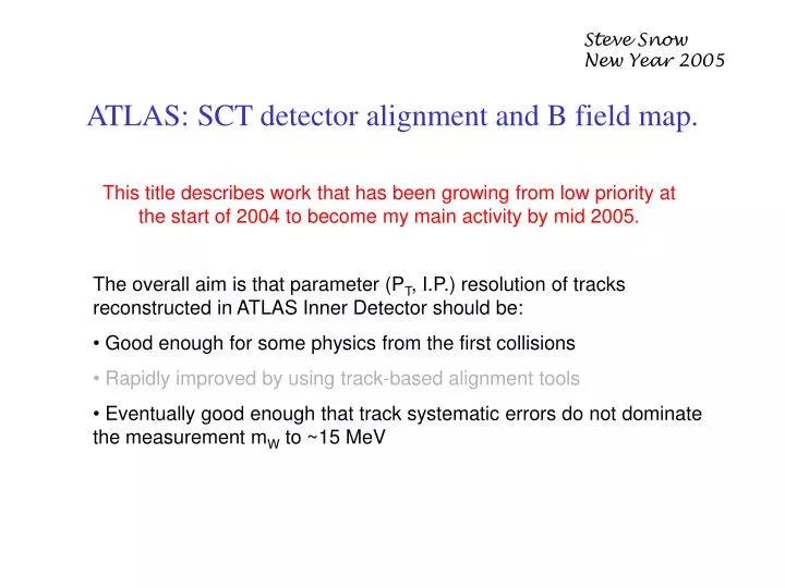
Steve Snow New Year 2005 ATLAS: SCT detector alignment and B field map. This title describes work that has been growing from low priority at the start of 2004 to become my main activity by mid 2005. • The overall aim is that parameter (PT, I.P.) resolution of tracks reconstructed in ATLAS Inner Detector should be: • Good enough for some physics from the first collisions • Rapidly improved by using track-based alignment tools • Eventually good enough that track systematic errors do not dominate the measurement mW to ~15 MeV
Initial Alignment I have been promoting the idea making an initial SCT alignment based on conventional surveys. This is a backup / alternative to the Oxford plan for an X-ray survey combined with FSI monitoring. The accuracy of the SCT endcap as built, and as surveyed is now becoming clear Intrinsic resolution of SCT detector; 22 mm (just under pitch/12). Detector positions in module; build 4 mm , survey 1 mm (Joe's talk). Location holes in module; build 10 mm , survey 3 mm. Module mounting pins on disc; build 100 mm , survey 10 mm. Discs in support cylinder; build 200 mm , survey 100 mm. Hole to pin clearance; <10 mm . Stability of mounting pins on disc; 20 - 50 mm . (temperature, moisture,bending ) If we can improve on disc-to-disc alignment (FSI or tracks) and the stability is at the better end of the range, then we could make a good alignment, similar to intrinsic detector resolution, from surveys on day 1.
Alignment - To do Collect and understand all module survey data ( 2000 modules) Already going into SCT database. Joe knows how to extract it. Module surveys done at several assembly sites; find and remove site-specific biases. Some already known. Collect and understand all disc survey data. ( 18 discs x 264 pins ) Sent to me from Liverpool and NIKHEF. So far discs 9c and 8c. Better understand disc stability, if there is an opportunity. Find/adapt/write software to make optimal use of multiple, over-constrained surveys. SIMULGEO ?
Module survey biases Correlation between Manchester and Liverpool surveys of the same module.
Disc survey data Displacement of pins from their nominal positions, Outer and Middle rings, Primary and Secondary pins.
Magnetic field map • Aim to make a map that is accurate to 1 part in 2000. • Map error will contribute to track momentum scale error. Important for mW. • Method is to combine: • Simulation with TOSCA (Bergsma), Mermaid (Voroijtsov), FlexPDE. • Mapping of field shape with Hall probes by Bergsma et al at CERN. • Monitoring of field strength with NMR probes throughout lifetime of Atlas. • Fitting with functions that obey Maxwell and use minimum number of parameters.
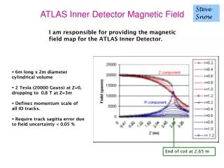
Toroid and Solenoid This picture shows the field strength in a slice of Atlas at Z=0. We are only interested in the solenoid; the small red spot at R<1m. Influence of the toroid through the TileCal is small not zero.
95% of the field is directly due to the current in the coil Coil Field shape. The field is very non-uniform at the ends of the coil; the Z component drops off and the R component rises sharply at z=2.65 m. Also plotted is the bending power per unit of radial travel for straight tracks from the origin; Bz-BR.Z/R .
Magnetisation field shape The field due to the magnetised iron is only 5% of the total. It is a slowly changing function of Z because the iron TileCal is relatively far from the Inner Detector.
Field fit approach • Build up fit from sum of basis fields: • Long-thin coil in vacuum (5mm longer, 5mm thinner than best estimate of real coil). • Short-fat coil in vacuum (5mm shorter, 5mm fatter). • Use a mixture of these two, with scale factors for length and field strength to fit the field due to the real coil. Allow the real coil to be offset and tilted with respect to the coordinate system of the mapping machine. Use same offset and tilt for both. • Few terms of Fourier-Bessel series to represent magnetisation field. Also allow this to have tilt and offset, maybe different from coil fields ? • Few non-cylindrical terms, not chosen yet. May represent non-circular coil, offset of coil from TileCal, ... John Hart investigating.
Test of aspect ratio fit. MINUIT fit. Three parameters; B_scale, L_scale, AR_mix. Dummy data is a field due to coil only with exactly the expected dimensions. Minimise |Bfit - Bdata|, summed over all grid points within the tracker active volume. Result is B_scale = 1.000005, L_scale= 0.999989, AR_mix=0.49979. r.m.s. residual is 0.16 gauss. As usual the only difficulty is near the coil end. Error could be reduced by generating new basis field which bracket the fit value more closely.
Mapper specification The specification that we arrive at depends on assumptions about how the machine will work. We assumed a structure like this: Typical positioning accuracies required are 0.3 mm for X, Y and Z survey of machine relative to tracker. (Presumably the sum of two surveys, mapper-to-rails and tracker-to-rails.) Rail sag and radial position of probes on arm require similar 0.2 mm accuracy. Typical angular accuracies required are 0.25 milliradians for rail tilt, axle tilt relative to Z axis, probes tilt relative to axle. Typical Hall probe accuracies required are 1 part in 10000 scale calibration, 4 parts in 10000 linearity.
Fourier Bessel fit I have has no success in getting a good fit to the coil field with the Fourier Bessel series. However the magnetisation field can be fitted well with only a few terms:
NMR probe locations NMR PROBES INSTALLED AT PHI=45,135,235, 315 DEGRES. 8A ATLAS SIDE A IP RAILS 9A CABLES ARE ROUTED AT Z=0 TO SECTOR 8A FOR THE TWO PROBES ABOVE THE RAILS AND 9A FOR THE TWO PROBES BELOW THE RAILS.
B field - To do Purchase rad hard NMR probes and cables. Jan/Feb 05. Find best QA tests of NMR system in absence of B field. Demonstrate that it works with chosen cables. April 05. Install NMR system. Aug/Sept 05. Modify field fit software to include - more Fourier-Bessel terms, non-regular grid, other mapping machine geometries, NMR probes in fit. Iterate on mapping machine specifications with Bergsma. Field map (solenoid on, all iron present, toroids may be off). Jan 06.
Self; 40% increasing to 70%, Soon-to-be-appointed e-science RA; 70% (other 30% on track quality monitoring) Some technical support on NMR (electronics) and possibly on mapping machine (mechanics/control). Effort Finally The end is in sight. By the end of this year the cavern will be crammed with detector and there will be nothing to watch on this webcam.