Download
1 / 24
240 likes | 356 Vues
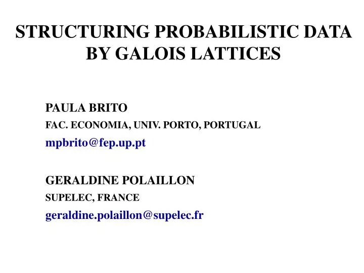
STRUCTURING PROBABILISTIC DATA BY GALOIS LATTICES. PAULA BRITO FAC. ECONOMIA, UNIV. PORTO, PORTUGAL mpbrito@fep.up.pt GERALDINE POLAILLON SUPELEC, FRANCE geraldine.polaillon@supelec.fr. GROUP. INSTRUCTION. FOOTBALL. 1. Students. Pr(0.08), Sec(0.88), Sup(0.03).

E N D
STRUCTURING PROBABILISTIC DATA BY GALOIS LATTICES PAULA BRITO FAC. ECONOMIA, UNIV. PORTO, PORTUGAL mpbrito@fep.up.pt GERALDINE POLAILLON SUPELEC, FRANCE geraldine.polaillon@supelec.fr
GROUP INSTRUCTION FOOTBALL 1 Students Pr(0.08), Sec(0.88), Sup(0.03) yes (0.51), no(0.49), no_ans (0.01) 2 Retired Pr(0.92), Sec(0.05), Sup(0.03) yes (0.12), no(0.88) 3 Employed Pr(0.59), Sec(0.39), Sup(0.02) yes (0.22), no(0.78) 4 Small independents Pr(0.62), Sec(0.31), Sup(0.07) yes (0.32), no(0.67), no_ans (0.01) 5 Housewives Pr(0.93), Sec(0.07) yes (0.10), no(0.90) 6 Intermediate executives Pr(0.17), Sec(0.50), Sup(0.33) yes (0.26), no(0.73), no_ans (0.01) 7 Industrial workers Pr(0.73), Sec(0.27), Sup(0.01) yes (0.40), no(0.60) 8 Intellectual/Scientific Executives Sec(0.01), Sup(0.99) yes (0.22), no(0.78) 9 Other Pr(0.72), Sec(0.229), Sup(0.07) yes (0.19), no(0.80), no_ans (0.01) 10 Manager / Independent Profession Sec(0.02), Sup(0.98) yes (0.28), no(0.70), no_ans (0.02) 11 Businessmen Pr(0.08), Sec(0.33), Sup(0.58) yes (0.42), no(0.58)
Outline • Probabilistic data • Galois connections • Lattice construction • Application • Conclusion and perspectives
Probabilistic data A modal variableYon a set E ={1, 2,…} with domain O = {y1, y2, …, yk} is a mapping Y : EM(O) from E into the family M(O) of all distributions on O, with values Y() = .
Probabilistic data DEFINITION A modalevent is a statement of the form e = [Y() R {y1(p1), y2(p2), …, yk(pk)}] where O = {y1, y2, …, yk} is the domain of Y, and pj is the probability, frequency or weight of yj. It is not imposed that p1+ p2+…+ pk= 1. R is a relation on the set of distributions on O.
We shall consider the following relations: i) “~” such that [Y() ~ {y1(p1),…, yk(pk)}] is true iff ii) “” such that [Y() {y1(p1),…, yk(pk)}] is true iff iii) “” such that [Y() {y1(p1),…, yk(pk)}] is true iff
A modal objectis a conjunction of modal events. Each individual E is described by a modal probabilistic object: Let S be the set of all modal objects defined on variables Y1, ..., Yp
Galois Connections THEOREM 1 The couple of mappings fu: S P(E) s extE s = {w E : s(w) s } gu : P(E) S {w1, … ,wk} with tji = Max{pji(wh), h=1,...,k}, j=1,…,ki, i=1,..., p form a Galois connection between (P(E),) and (S ,).
Sex Instruction G1 Masc.(0.4), Fem.(0.6) Prim.(0.3), Sec.(0.4), Sup.(0.3) G2 Masc.(0.1), Fem.(0.9) Prim.(0.1), Sec.(0.2), Sup.(0.7) G3 Masc.(0.8), Fem.(0.2) Prim.(0.2), Sec.(0.3), Sup.(0.5) G4 Masc.(0.5), Fem.(0.5) Prim.(0.3), Sec.(0.2), Sup.(0.5) Example Let A = {G1, G2} gu(A) = fu(gu(A)) = {G1, G2}
THEOREM 2 The couple of mappings fi : S P(E) s extE s ={w E : s(w) s } gi : P(E) S {w1, … ,wk} with tji = Min{pji(wh), h=1,...,k}, j=1,…,ki, i=1,..., p form a Galois connection between (P(E),) and (S,).
Sex Instruction G1 Masc.(0.4), Fem.(0.6) Prim.(0.3), Sec.(0.4), Sup.(0.3) G2 Masc.(0.1), Fem.(0.9) Prim.(0.1), Sec.(0.2), Sup.(0.7) G3 Masc.(0.8), Fem.(0.2) Prim.(0.2), Sec.(0.3), Sup.(0.5) G4 Masc.(0.5), Fem.(0.5) Prim.(0.3), Sec.(0.2), Sup.(0.5) Example Let B = {G2, G3}. gi(B) = fi(gi(B)) = {G2, G3, G4}
THEOREM 3 Let (fu,gu) be the Galois connection in theorem 1. If and we define s1 s2 = with tji = Max{rji, qji}, j=1,…,ki, i=1,..., p and s1 s2 = with zji = Min{rji, qji}, j=1,…,ki, i=1,..., p. The set of concepts, ordered by (A1, s1)(A2, s2) A1 A2 is a lattice where : inf (( A1, s1 ),( A2 , s2 )) = ( A1 A2 ,(gu o fu)( s1 s2 )) sup (( A1, s1 ),( A2 , s2 )) = ((fu o gu)(A1 A2), s1 s2 ) This lattice will be called “union lattice”.
The set of concepts, ordered by (A1, s1)(A2, s2) A1 A2 • is a lattice where : • inf (( A1, s1 ),( A2 , s2 )) = ( A1 A2 ,(gu o fu)( s1 s2 )) • sup (( A1, s1 ),( A2 , s2 )) = ((fu o gu)(A1 A2), s1 s2 ) • This lattice will be called “union lattice”.
THEOREM 4 Let (fi,gi) be the Galois connection in theorem 2. If and we define s1 s2 = with tji = Min{rji, qji}, j=1,…,ki, i=1,..., p and s1 s2 = with zji = Max{rji, qji}, j=1,…,ki, i=1,..., p.
The set of concepts, ordered by(A1, s1)(A2, s2) A1 A2 is a lattice where : inf (( A1, s1 ),( A2 , s2 )) = ( A1 A2 ,(gi o fi)( s1 s2 )) sup (( A1, s1 ),( A2 , s2 )) = ((fi o gi)(A1 A2), s1 s2 ) This lattice will be called “intersection lattice”.
Lattice construction First step : find the set of concepts Ganter's algorithm (Ganter & Wille, 1999) : searches for closed sets by exploring the closure space in a certain order. To reduce computational complexity, we look for the concepts exploring the set of individuals.
Second Step : Graphical representation Definition of a drawing diagram algorithm Principle : Use graph theory When we insert a new concept in the graph, we explore all nodes of the existing graph only once. The complexity of this algorithm is o(N²).
Tinnitus Headache Blood Pressure Name Often Seldom Often Seldom High Normal Low Ann 0.8 0.2 0.9 0.1 0.8 0.2 0.0 Bob 1.0 0.0 0.0 1.0 0.6 0.4 0.0 Chris 1.0 0.0 0.1 0.9 0.9 0.1 0.0 Doug 0.3 0.7 0.7 0.3 0.0 0.6 0.4 Eve 0.6 0.4 0.7 0.3 0.0 0.8 0.2 Comparison (Herrman & Hölldobler (1996) ) c : {{Ann, Bob, Chris}{Tinnitus (often), Blood Pressure (high)}, =0.85, =0.11} From the intersection concept lattice: a7 i = [Tinnitus {often(0.8), seldom(0.0)}] ^ [Blood Pressure{high(0.6), normal (0.1), low(0.0)}] ext (a7 i) = {Ann, Bob, Chris} From the union concept lattice: a7u = [Tinnitus£ {often(1.0), seldom(0.2)}] ^ [Blood Pressure£ {high(0.9), normal (0.4),low(0.0)}] ext (a7 u) = {Ann, Bob, Chris}
Employment data Variables : • Marital status • Education • Economic activity (CEA) • Profession • Searching employment • Full/part time. 12 Groups : Gender Age group
a19 = [Status£ {widow(0.01) divorced(0.14) married(0.94) single(0.71)}] ^ [CEA£ {agriculture, cattle, hunt, forestry & fishing (0.10), construction(0.26), other services(0.34), real estate, renting & business activities(0.06), wholesale and retail trade, repairs(0.18), public administration(0.09), manufacturing(0.38), transport, storage & communication(0.08), hotels & restaurants(0.10), electricity, gas & water(0.02), financial intermediation(0.02), mining & quarrying(0.01)}] ^ [Profession£ {skilled agriculture and fishery workers(0.08), elementary occupations(0.19), plant and machine operators and assemblers(0.14), craft and related trade workers(0.42), professionals(0.11), clerks(0.14), service, shop & market sales workers(0.28), technicians and associate professionals(0.10), legislators, senior officers and managers(0.13),armed forces(0.02)}] ^ [Education£ {without education(0.05), primary(0.69), secondary(0.42), superior(0.16)}] ^ [Searching£ {search_no(0.99), search_yes(0.04)}] ^ [Part/Full£ {part time(0.11), full time(0.98)}] Ext a19 = {Men 15-24, Men 35-44, Men 45-54, Women 15-24, Women 25-34, Women 35-44}
Lattice simplification DEFINITION (Leclerc, 1994) Let(P,) be an ordered set. An element x P is said to be sup-irreducible if it is not the supremum of a finite part of P not containing it. Dually, we define an inf-irreducible element. The notion of irreducible elements may be used to simplify the lattice graphical representation (Duquenne, 1987), (Godin et al, 1995).
Conclusion and Perspectives • Extension of lattice theory to deal directly with probabilistic data – no prior transformation • Two kinds of Galois connections • Algorithm to construct the Galois lattices on these data • Limitation : size of the resulting lattice • Take order into account • Simplification of the lattice