Download
1 / 29
300 likes | 579 Vues
Using the recombining binomial tree to pricing the interest rate derivatives: Libor Market Model. 何俊儒 2007/11/27. Agenda. The reason why I choose this issue The property of the LIBOR Market Model (LMM) Review of other interest rate models The procedures which how to complete my paper.

E N D
Using the recombining binomial tree to pricing the interest rate derivatives: Libor Market Model 何俊儒 2007/11/27
Agenda • The reason why I choose this issue • The property of the LIBORMarket Model (LMM) • Review of other interest rate models • The procedures which how to complete my paper
Reasons • The lattice based approach provides an efficient alternative to Monte Carlo Simulation • It provides a fast and accurate method for valuation of path dependent interest rate derivatives under one or two factors • The LIBORMarket Model is expressed in terms of the forward rates that traders are used to working with
The property of LIBOR Market Model • Brace, Gatarek and Musiela (BGM) (1997) • Jamshidian (1997) • Miltersen, Sandmann and Sondermann (1997) • All of above propose an alternative and it is known as the LIBOR market model (LMM) or the BGM model • The rate where we use is the forward rate not the instantaneous forward rate
The property of LIBOR Market Model • We can obtain the forward rate by using bootstrap method • It is consistent with the term structure of the interest rate of the market and by using the calibration to make the volatility term structure of forward rate consistent • Assume the LIBOR has a conditional probability distribution which is lognormal • The forward rate evolution process is a non-Markov process • The nodes at time n is (see Figure 1)
The property of LIBOR Market Model • It results that it is hard to implement since the exploding tree of forward and spot rates • When implementing the multi-factor version of the LMM, tree computation is difficult and complicated, the Monte Carlo simulation approach is a better choice
Review of other interest rate models • Standard market model • Short rate model • Equilibrium model • No-arbitrage model • Forward rate model
The standard market models The Black’s models for pricing interest rate options • Assume that the probability distribution of an interest rate is lognormal • It is widely used for valuing instruments such as • Caps • European bond options • European swap options
The standard market models • The lognormal assumption has the limitation that doesn’t provide a description of how interest rates evolve through time • Consequently, they can’t be used for valuing interest rate derivatives such as • American-style swaption • Callable bond • Structured notes
Short-rate models • The alternative approaches for overcoming the limitations we met in the standard market models • This is a model describing the evolution of all zero-coupon interest rates • We focus on term structure models constructed by specifying the behavior of the short-term interest rate, r
Short-rate models • Equilibrium models • One factor models • Two factor models • No-Arbitrage models • One factor models • Two factor models
Equilibrium models • With assumption about economic variables and derive a process for the short rate, r • Usually the risk-neutral process for the short rate is described by an Ito process of the form dr = m(r)dt + s(r)dz where m is the instantaneous drift s is the instantaneous standard deviation
Equilibrium models • The assumption that the short-term interest rate behaves like a stock price has a cycle, in some period it has a trend to increasing or decreasing • One important property is that interest rate appear to be pulled back to some long-run average level over time • This phenomenon is known as mean reversion
Mean Reversion Interest rate HIGH interest rate has negative trend Reversion Level LOW interest rate has positive trend
Equilibrium modelstwo factor model • Brennan and Schwartz model (1979) • have developed a model where the process for the short rate reverts to a long rate, which in turn follows a stochastic process • Longstaff and Schwartz model (1992) • starts with a general equilibrium model of the economy and derives a term structure model where there is stochastic volatility
No Arbitrage models • The disadvantage of the equilibrium models is that they don’t automatically fit today’s term structure of interest rates • No arbitrage model is a model designed to be exactly consistent with today’s term structure of interest rates
No Arbitrage models • The Ho-Lee model (1986) dr = q(t )dt + sdz • The Hull-White (one-factor) model (1990) dr = [q(t ) – ar ]dt + sdz • The Black-Karasinski model (1991) • The Hull-White (two-factor) model (1994) u with an initial value of zero
Summary of the models we mentioned • A good interest rate model should have the following three basic characteristics: • Interest rates should be positive • should be autoregressive • We should get simple formulate for bond prices and for the prices of some derivatives • A model giving a good approximation to what observed in reality is more appropriate than that with elegant formulas
Two limitations of the models we mentioned before • Most involve only one factor (i.e., one source of uncertain ) • They don’t give the user complete freedom in choosing the volatility structure
Forward rate model • HJM model • BGM model
HJM model • It was first proposed in 1992 by Heath, Jarrow and Morton • It gives up the instantaneous short rate which we common used and adapts the instantaneous forward rate • We can express the stochastic process of the zero coupon bond as follows:
HJM model • According to the relation between zero coupon bond and forward rate, we can obtain • Hence, we can infer the stochastic process of the forward rate as follows where
HJM model • If we want to use HJM model to price the derivative, we have to input two exogenous conditions: • The initial term structure of forward rate • The volatility term structure of forward rate
The procedures of completing the paper • According to HSS(1995) to construct the recombining binomial tree under the LIBOR market model • Using the tree computation skill to price the interest rate derivatives, such as • Caps, floors and so on • Bermudan-style swaption • Solving the nonlinearity error of the tree and calibration the parameter to be consistent with the reality