Download
1 / 26
280 likes | 466 Vues
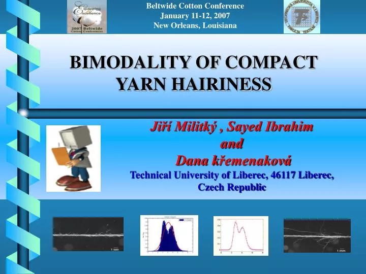
Beltwide Cotton Conference January 11-12, 2007 New Orleans, Louisiana. BIMODALITY OF COMPACT YARN HAIRINESS. Jiří Militký , Sayed Ibrahim and Dana k řemenaková Technical University of Liberec, 46117 Liberec, Czech Republic. Introduction.

E N D
Beltwide Cotton Conference January 11-12, 2007 New Orleans, Louisiana BIMODALITY OF COMPACT YARN HAIRINESS Jiří Militký , Sayed Ibrahim and Dana křemenaková Technical University of Liberec, 46117 Liberec, Czech Republic
Introduction Hairiness is considered as sum of the fibre ends and loops standing out from the main compact yarn body The most popular instrument is the Uster hairiness system, which characterizes the hairiness by H value, and is defined as the total length of all hairs within one centimeter of yarn. The system introduced by Zweigle, counts the number of hairs of defined lengths. The S3 gives the number of hairs of 3mm and longer. The information obtained from both systems are limited, and the available methods either compress the data into a single vale H or S3, convert the entire data set into a spectrogram deleting the important spatial information. Other less known instruments such as Shirley hairiness meter or F-Hairmeter give very poor information about the distribution characteristics of yarn hairiness. Some laboratory systems dealing with image processing, decomposing the hairiness into two exponential functions (Neckar,s Model), this method is time consuming, dealing with very short lengths.
Outlines • Investigating the possibility of approximating the yarn hairiness distribution by a mixture of two Gaussian distributions. • Complex characterization of yarn hairiness data in time and frequency domain i.e. describing the hairiness by: • - periodic components • - Random variation • - Chaotic behavior
Ring-Compact Spinning 1)Draft arrangement 1a) Condensing element 1b) Perforated apron VZ Condensing zone 2) Yarn Balloon with new Structure 3) Traveler, 4) Ring 5) Spindle, 6) Ring carriage 7) Cop, 8) Balloon limiter 9) Yarn guide, 10) Roving E) Spinning triangle of compact spinning
Experimental Part &Method of Evaluation • Three cotton combed yarns of counts 14.6, 20 and 30 tex were produced on three commercial compact ring spinning machines. The yarns were tested on Uster Tester 4 for 1 minute at 400 m/min. • The raw data from Uster tester 4 were extracted and converted to individual readings corresponding to yarn hairiness, i.e. the total hair length per unit length (centimeter).
Investigation of Bimodality of yarn Hairiness Number and width of bars affect the shape of the probability distribution The question is how to optimize the width of bars for better evaluation? Hair Diagram Histogram (83 columns) Normal Dist. fit Gaussian curve fit (20 columns) Smooth curve fit
Basics of Probability density function I • The area of a column in a histogram represents a piecewise constant estimator of sample probability density. Its height is estimated by: • Where is the number of sample • elements in this interval • and is the length • of this interval. • Number of classes • For all samples is N= 18458 and M=125 h = 0.133
Kernel density function The Kernel type nonparametric of sample probability density function Kernel function : bi-quadratic - symmetric around zero - properties of PDF Optimalbandwidth : h 1. Based on the assumptions of near normality 2. Adaptive smoothing 3. Exploratory (local hj ) requirement of equal probability in all classes h = 0.1278
Bi-modal distributionTwo Gaussian Distribution MATLAB 7.1 RELEASE 14 The bi-modal distribution can be approximated by two Gaussian distributions, Where , are proportions of shorter and longer hair distribution respectively, , are the means and , are the standard deviations. H-yarn Program written in Matlab code, using the least square method is used for estimating these parameters.
Bi-modality of Yarn HairinessMixed Gaussian Distribution The frequency distribution and fitted bimodal distribution curve
Analysis of Results Check the type of Distribution Bimodality parametric • Mixture of distributions estimation and likelihood ratio test • Test of significant distance between modes (Separation) Bimodality nonparametric: • kernel density (Silverman test) • CDF (DIP, Kolmogorov tests) • Rankit plot unimodal Gaussian smoother closest to the x and the closest bimodal Gaussian smoother
Basic Distribution function definitions In general, the Dip test is for bimodality. However, mixture of two distributions does not necessarily result in a bimodal distribution.
Analysis of Results IMixture of Gauss distributions Probabilitydensity function (PDF) f (x), Cumulative Distribution Function (CDF) F (x), and Empirical CDF (ECDF) Fn(x) Unimodal CDF: convex in (−∞, m), concave in [m, ∞) Bimodal CDF: one bump Let G∗ = arg min supx |Fn(x) − G(x)|, where G(x) is a unimode CDF. Dip Statistic: d = supx |Fn(x) − G∗(x)| Dip Statistic (for n= 18500): 0.0102 Critical value (n = 1000): 0.017 Critical value (n = 2000): 0.0112
Analysis of Results IIDip Test Dip test statistics: It is the largest vertical difference between the empirical cumulative distribution FE and the Uniform distribution FU Points A and B are modes, shaded areas C,D are bumps, area E and F is a shoulder point This test is actually identification of mixed mixture of normal distribution, is only rejecting unimodality
Analysis of Results IIILikelihood ratio test The single normal distribution model (μ,σ), the likelihood function is: Where the data set contains n observations. The mixture of two normal distributions, assumes that each data point belongs to one of tow sub-population. The likelihood of this function is given as: The likelihood ratio can be calculated from Lu and Lb as follows:
Significance of difference of means Analysis of Results V • Two sample t test of equality of means • T1 equal variances • T2 different variances
PDF and CDF Analysis of Results VI Kernel density estimator: Adaptive Kernel Density Estimator for univariate data. (choice of band width h determines the amount of smoothing. If a long tailed distribution, fixed band width suffer from constant width across the entire sample. For very small band width an over smoothing may occur ) MATLAB AKDEST 1D- evaluates the univariate Adaptive Kernel Density Estimate with kernel
Parameter estimation of • mixture of two Gaussians model
Complex Characterization of Yarn Hairiness • The yarn hairiness can be also described according to the: • Random variation • Periodic components • Chaotic behavior • The H-yarn program provides all calculations and offers graphs dealing with the analysis of yarn hairiness as Stochastic Process.
Basic definitions of Time Series • Since, the yarn hairiness is measured at equal-distance, the data obtained could be analyzed on the base of time series. • A time series is a sequence of observations taken sequentially in time. The nature of the dependence among observations of a time series is of considerable practical interest. • First of all, one should investigate the stationarity of the system. • Stationary model assumes that the process remains in equilibrium about a constant mean level. The random process is strictly stationary if all statistical characteristics and distributions are independent on ensemble location. • Many tests such as nonparametric test, run test, variability (difference test), cumulative periodogramconstruction are provided to explore the stationarity of the process.
Stationarity testPeriodogram System A 14.6 tex For characterization of independence hypothesis against periodicity alternative the cumulative periodogram C(fi) can be constructed. For white noise series (i.i.d normally distributed data), the plot of C(fi) against fiwould be scattered about a straight line joining the points (0,0) and (0.5,1). Periodicities would tend to produce a series of neighboring values of I(fi) which were large. The result of periodicities therefore bumps on the expected line. The limit lines for 95 % confidence interval of C(fi) are drawn at distances. System B System C
Time Domain Analysis Autocorrelation Simply the Autocorrelation function is a comparison of a signal with itself as a function of time shift. Autocorrelation coefficient of first order R(1) can be evaluatedas System A System B System C For sufficiently high L is first order autocorrelation equal to zero
Frequency domain The Fast Fourier Transformation is used to transform from time domain to frequency domain and back again is based on Fourier transform and its inverse. There are many types of spectrum analysis, PSD, Amplitude spectrum, Auto regressive frequency spectrum, moving average frequency spectrum, ARMA freq. Spectrum and many other types are included in Hyarn program. System A System C System B
Fractal DimensionHurst Exponent The cumulative of white Identically Distribution noise is known as Brownian motion or a random walk. The Hurst exponent is a good estimator for measuring the fractal dimension. The Hurst equation is given as . The parameter H is the Hurst exponent. The fractal dimension can be measured by 2-H. In this case the cumulative of white noise will be 1.5. More useful is expressing the fractal dimension 1/H using probability space rather than geometrical space. System A System B System C
Summery of results of ACF, Power Spectrum and Hurst Exponent
Conclusions • Preliminary investigation shows that the yarn hairiness distribution can be fitted to a bimodal model distribution. • The yarn Hairiness can be described by two mixed Gaussian distributions, the portion, mean and the standard deviation of each component leads to deeper understanding and evaluation of hairiness. • This method is quick compared to image analysis system, beside that, the raw data is obtained from world wide used instrument “Uster Tester”. • The Hyarn system is a powerful program for evaluation and analysis of yarn hairiness as a dynamic process, in both time and frequency domain. • Hyarn program is capable of estimating the short and long term dependency.