Download
1 / 1
10 likes | 104 Vues
Detection of Giant pulses from pulsar PSR B0950+08. Smirnova T.V. tania@prao.ru Pushchino Radio Astronomy Observatory of ASC FIAN.

E N D
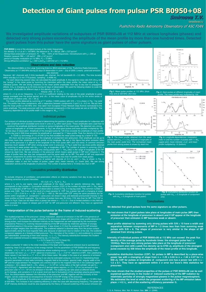
Detection of Giant pulses from pulsar PSR B0950+08 Smirnova T.V. tania@prao.ru Pushchino Radio Astronomy Observatory of ASC FIAN We investigated amplitude variations of subpulses of PSR B0950+08 at 112 MHz at various longitudes (phases) and detectedvery strong pulses exceeding the amplitude of the mean profileby more than one hundred times. Detected giant pulsesfrom this pulsar have the same signature asgiant pulsesof other pulsars. PSR B0950 isone of the strongest pulsars at the meter frequencies, flux density:S = 2Jy atf = 102 MHz, the distance is: R = 262 pc, DM = 2.97 pc/cm3 Strong linear polarizationof emission: PL~ 70% - 100% at low frequencies, microstructure with tµ = 200 µs Rotation measureRM = 1.35 rad/m2 , DM = 2.97pc/cm3, period of Faradey modulation at 112 MHz: PF = 15 MHz Strong diffractive scintillation: tdif > 300 s and fdif = 220 kHz at f = 112 MHz. Observations and data reduction We obtained data on the Large Scanning Antenna (BSA telescope) of the Pushchino Radio Astronomy Observatory at 111.846 MHz during 22 days of observation in June – July of 2009. Linearly polarized emission was received. Receiver:461channels with5KHz bandwidth per channel, the full bandwidth В = 2.3MHz. The time duration within one day is 3.3 min (770 pulses), sampling – 0.4096 ms. For each observing session (day) we calculated the peak amplitude A, the signal-to-noise ratio S/N (A/σN) and the “energy” in the mean pulse by summing the intensities within the mean profile, the mean value of σNforindividual pulses. We see strong variations of the mean profile amplitudes from day to day due to propagation effects: A/σN is changing up to 44 times during 22 days of observation. We used the following relation to scale the pulse peak amplitudes for different days in flux-density units (Jy): A(t)[Jy] =A(t) · S · k /< A >, where S = 2 Jy at our frequency, k = 14.9 is a coefficient relating to the ratio of the peak amplitude to pulse energy averaged over the pulsar period, and <A> is the mean value of amplitudes A(t) for the entire series of observation in relative units, <A> = 30 Jy. The mean profile obtained by summing of 17 profiles (13000 pulses) with S/N > 14 is shown in Fig. 1 by solid line. The profile has three components, with a separation between components 2 and 3, Δ = 6.2 ms. We put here also the mean profile at 430 MHz (thin line) taken from European Pulsar Network Data Archive normalized to the same amplitude. The weak precursor with two unresolved components in the main pulse we see at 430 MHz. The frequency dependence of the profile width in this range is: W0.5 ~ f -0.35. Fig.1. Mean pulse profiles at 112 MHz (thick line) and at 430 MHz (thin line) Fig. 2. Giant pulses at different longitudes of mean profile. The mean profile was multiplied by 100. Individual pulses Our analysis of individual pulses consisted of determining the positions (phases) and amplitudes for subpulses with a peak amplitude which exceeded some level in units of σN within each pulse. These amplitudes were used then to construct the amplitude distribution function at various longitudes of the mean pulse. We detected very strong pulses at longitudes of all three components. In Fig 2 we show giant pulses and mean profiles multiplied by 100 for two days of observation. Amplitude of the strongest pulse by 120 times exceeds the amplitude of mean profile for this day and in 508 times exceeds the amplitude of averaged for 17 days profile. Peak flux density of this pulse is 15240 Jy and energy of it is 81240 Jy*ms that exceeds the mean pulse energy by a factor of 153. We have rare but strong pulses at the longitude of component one (precursor), their amplitude can be up to 490 times more than amplitude of mean profile at this longitude. We see in this figure that when emission takes place at the precursor it is absent at the longitude of the main pulse (MP) and vice-versa. In common emission becomes much weaker in MP when strong pulses exist in precursor. In Fig.3 (solid line) we show profile obtained by summing of weak pulses with 6σN > I > 3σN at longitudes of MP. The number of pulses in summing (233) is about the same as for profile selecting only strong pulses with I > 10σN (262) in the range of longitudes of the MP (shown by dash line). We see emission in the precursor which means weak pulses in MP don’t influence it. The shape of profile here has also two components and the same width as for MP. The width of MP and separation between components for profile from strong pulses are 1.5 times less than for profile from weak pulses. Longitude analysis of intensity variations of pulses with discrete of 0.4 ms and I > 5σN is shown in Fig. 4: modulation index m and the number of pulses (upper plot); mean intensity <I> (lower plot). We see strong modulation activity at the longitudes of precursor. The number of pulses here is 10 times less than in MP. Fig. 3. The mean profile obtained from the weak pulses with 6 σN > I > 3 σN realized at longitudes of the main pulse (solid line). The normalized mean profile from strong pulses is shown by dash line. Fig. 4. Longitude dependences: modulation index m and the number of pulses with I > 5σN (upper plot); mean intensity <I>(l) and mean profile multiplied by 10 (bottom) Cumulative probability distribution To excludeinfluence of scintillation and polarization effects on intensity variations from day to day we did the following correction of pulse intensities: I(t) =In(t) ·σ0N · A0/(σnN · An), where σ0N and A0 are sigma noise and amplitude of the mean profile for specific reference day, index n corresponds to day number n. Cumulative distribution function (CDF) of the number of pulses with I > 5σN taken place at longitudes of MP from 17 days of observation is shown in Fig. 5 in log-log scale. The common number of pulses was 3385. Two lines are the result of a least-squares fit. CDF has a power law with a changing of slope from n = -1.25 ± 0.04 to n = -1.84 ± 0.07 for I > 600 Jy. We also build CDF using the same procedure but for pulses within longitudes of component 1 (precursor) we chose 5 days and detected pronounced intensity in the mean profiles at these longitudes. The number of pulses here was 30 times (119) less than for MP. This CDF is shown in Fig.6. Data can be fitted within a power law where n = -1.5 ± 0.1. Due to limited statistics in this field we can't conclude that slopes of steeper part of CDF for MP and precursor are different: they have an agreement within 3 σ error. Interpretation of the pulse behavior in the frame of induced-scattering model The studied properties of the precursor: strong modulation, absence of emission in the MP in the presence of powerful GPs in the precursor range, similarity of the precursors shape with that of the mean profile obtained for strong pulses, and increase the emission intensity at low frequencies are well explained by the mechanism proposed by Petrova [1], involving induced scattering of the MP emission by relativistic particles of strongly magnetized plasma in the pulsar magnetosphere. It was shown in [1] that the scattering of the MP emission occurs at larger heights than the initial pulse. The scattered radiation is directed away from the pulsar surface, approximately along the local magnetic field, and, because of aberration due to rotation of the star, the scattered component appears as a forward-shifted precursor. The intensities of the incident (I1) and scattered (I2) emission are redistributed, conserving of their total intensity: I = I1 + I2. The intensity redistribution between the incident (MP) and scattered emission is determined by eq. (11) from [1]: I1 = I(I10/I20)exp(-G)/(1+(I10/I20)exp(-G)) I2 = I/(1+(I10/I20)exp(-G)), where a subscript ‘0’ refers to the initial intensities of the beam and background emission due to spontaneous scattering. Here G is an efficiency of the energy transfer. For the parameters of PSR B0950+08 and frequency112 MHz,I10/I20 = 1010 и 1012for the distances where scattering occurs:r = 108и 109сm respectively. From observation we have: I2/I1 < = 2*10-3 (absence of precursor), I1/I2 < = 5.6*10-3(absence of MP), thensubstituting these values (1) we have G<= 17 и G>= 28 for these cases. We adopt in the case of an absence of emission the 2 σNlevel. The efficiency of scattering G can also be estimated using eq. (13) from [1]. Substituting these equation parameters of total radio luminosity, magnetic field at the surface, spectral index, angular width of the MP and the angle between the magnetic axis and the tangent to the magnetic field line in the scattering region at a distance r (for a dipole field θ = r/2rL, where rL= 1.2×109 cm is the radius of the light cylinder) we got G = 421(r[108сm])-8. Agreement with the values of G derived above requires r ≥ 1.5 × 108 cm (no emission in the precursor) and r ≤ 1.4 × 108 cm (no emission in the MP). The scattering can take place at different levels as G changes, and variations in G at a given level are due to fluctuations of the secondary-plasma parameters. Thus, the anticorrelation between the intensities of the precursor and MP, together with the similarity of their shapes, can be understood as consequence of transfer of the MP energy to the precursor. The relative amplitude of the precursor considerably increases, and it is three times stronger at 112 MHz than at 430 MHz. This increase in the scattering efficiency is often the case with decreasing frequency. The power law of GP intensity distribution could be also explained by the theory of induced scattering of the pulsar emission [2]. Fig. 6. Cumulative distribution function for pulses with I/σN > 5 (longitude of component one). Fig. 5. Cumulative distribution function for pulses with I/σN > 5 (longitude of main pulse). • Conclusions We detected that giant pulseshave the same signature as other pulsars. • We had shown that if giant pulses take place at longitudes of main pulse (MP) then emission at the longitude of precursor is absent and if GP appear at the longitude of precursor then emission in MP becomes weak or absent. Mean profile obtained by summing only strong pulses with S/N > 10 have a width and separation between components of MP in 1.5 times less than from summing weak pulses with S/N < 6. The shape of precursor is very similar to the shape of MP obtained from strong pulses. Intensity of individual pulses of PSR B0950+08 at 112 MHz can exceed the peak flux density of the average pulse by hundreds times: the strongest pulse hasI = 15240Jy. Rare but very strong pulses take place at the longitude of precursor (component one) with a peak flux density up to 5750 Jy, amplitude of the strongest pulse exceeds by 508 times the amplitude of the mean profile at this longitude. Cumulative distribution function (CDF) for pulses in MP is described by a piece-wise power law with a changing of slope from n = -1.25 ± 0.04 to n = -1.84 ± 0.07 for I > 600 Jy. CDF for pulses at longitudes of component one has a power law with n = -1.5 ± 0.1. They have an agreement within 3 σ error but there’s little statistics for precursor. • We have shown that the studied properties of the pulses of PSR B0950+08 can be well explained qualitatively in the model of induced scattering of the MP radiation by relativistic particles of strongly magnetized plasma in the pulsar magnetosphere. We estimated the level at which the proposed scattering of the MP emission takes place: r ≈ 0.1rL and of the scattering efficiency parameter G. REFERENCES 1. S. A. Petrova, Mon. Not. R. Astron. Soc. 384, L1 (2008). 2. S. A. Petrova, Astron. Astrophys. 424, 227 (2004).