Download
1 / 12
120 likes | 233 Vues
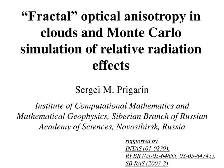
“Fractal” optical anisotropy in clouds and Monte Carlo simulation of relative radiation effects. Sergei M. Prigarin. Institute of Computational Mathematics and Mathematical Geophysics, Siberian Branch of Russian Academy of Sciences, Novosibirsk, Russia. supported by INTAS (01-0239),

E N D
“Fractal” optical anisotropy in clouds and Monte Carlo simulation of relative radiation effects Sergei M. Prigarin Institute of Computational Mathematics and Mathematical Geophysics, Siberian Branch of Russian Academy of Sciences, Novosibirsk, Russia supported by INTAS (01-0239), RFBR (03-05-64655, 03-05-64745), SB RAS (2003-2)
A hypothesis is made that optical anisotropy of clouds in the atmosphere can be implied not only by the shape and the orientation of scattering particles, but furthermore it can be a result of a random non-Poisson distribution of the particles in space. In that way even for water-drop clouds the optical medium can be appreciably anisotropic if spherical water drops particularly distributed in space. An admissible model for the spatial distribution can be obtained under assumption that particles are concentrated on a manifold of a dimension less then 3. That is an explanation of the term «fractal anisotropy».
The aims of the research:- to propose a mathematical description of the fractal anisotropy- to perform a Monte Carlo experiment to study probable radiation effects caused by fractal anisotropy in water-drop clouds
The following observations are the basis of the hypothesis: - distribution of scattering particles in a cloud can be non-Poisson,- fractal nature of spatial distributions for scattering particles in a cloud Publications on distribution of scattering particles in clouds:Kostinski, A. B., and A. R. Jameson, 2000: On the spatial distribution of cloud particles, J. Atmos. Sci., 57, P.901-915.A.B.Kostinski, On the extinction of radiation by a homogeneous but spatially correlated random medium, J.Opt. Soc. Am. A, August 2001, Vol.18, No.8, P.1929-1933Knyazikhin, Y., A. Marshak, W. J. Wiscombe, J. Martonchik, and R. B. Myneni, 2002: A missing solution to the transport equation and its effect on estimation of cloud absorptive properties, J. Atmos. Sci., 59, No.24, 3572-5385.Knyazikhin, Y., A. Marshak, W. J. Wiscombe, J. Martonchik, and R. B. Myneni, 2004: Influence of small-scale cloud drop size variability on estimation cloud optical properties, J. Atmos. Sci., (submitted).
Poisson distribution Non-Poisson anisotropic distributions:
A model of “fractal anisotropy” • Optically isotropic homogeneous media: • phase function g • single scattering albedo q • extinction coefficient • Fractal anisotropy: • phase function g • single scattering albedo q • extinction coefficient in the direction =(a,b,c): () = /{(a/cx)2+(b/cy)2+(c/cz)2}1/2, =(a,b,c), cxcycz=1
The range of a particle from point (0,0,0)to poin (x,y,z) in optically isotropic medium corresponds to the range from point (0,0,0) to point (cxx, cyy, czz )in anisotropic medium. Here cx,cy,czare compression coefficients for the compression directions OX,OY,OZ, cxcycz=1. • In general case there are 3 orthogonal compression directions with correspondent unit vectors e1,e2,e3 and compression coefficients c1,c2,c3, c1c2c3=1. In this case () = / T-1 , Where T is the compression tensor: T=c1e1e1T+c2e2e2T+c3e3e3T
Heuristic derivation of the model • A homogeneous optically isotropic scattering medium with extinction coefficient is concentrated in a whole space volume without empty spaces • Scattering medium with extinction coefficient /P is concentrated on a random homogeneous isotropic set S that covers portion P<1 of the space volume. The linear sizes of empty regions are small enough and uncorrelated. • P goes to zero; hence, the measure of S converges to zero as well (S is a fractal). • Instead of set S={(x,y,z)} we consider a setTS={T(x,y,z): (x,y,z)S}, where T is a compression tensor.
Numerical experiments (Monte Carlo simulation) What radiation effects can be caused by fractal anisotropy? For the numerical experiments we set: c2=c3=c1-1/2 c1 is the basic compression coefficient e1 is the basic compression direction
- visible range of wavelength; SSA=1; C1 cloud layer;- thickness: 250 m; ext. coeff.=0.02m-1 (optical depth = 5)- e1=(0,0,1): the basic compression direction is vertical red: optically isotropic medium, c1=1 green: vertically dense medium, c1=4 black: vertically rare medium, c1=0.25
- e1=(sin(Z),0,cos(Z)), where Z is the zenithal angle of the basic compression direction: Z=00,45,60,90 deg.
Angular distributions of downward radiation (the sun is in the zenith) Vertically dense medium: e1=(0,0,1), c1=4 Horizontally rare medium: e1=(1,0,0), c1=0.25 Isotropic medium