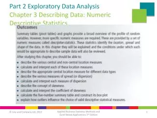
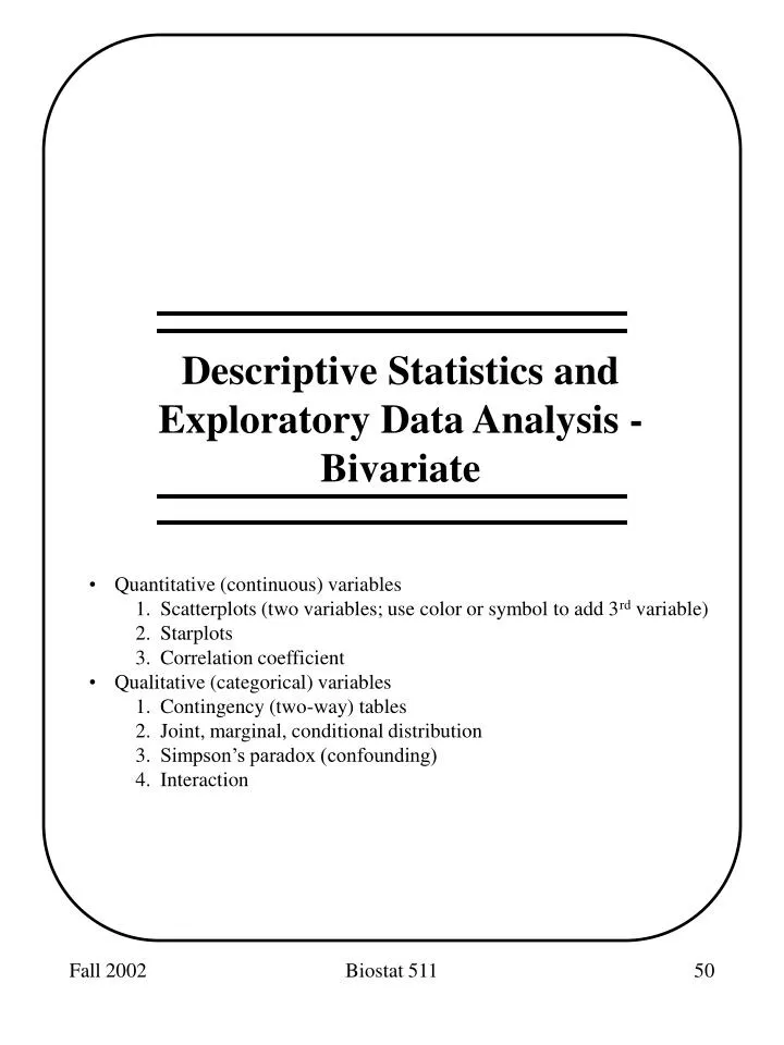
Descriptive Statistics and Exploratory Data Analysis - Bivariate

1. Descriptive Statistics and Exploratory Data Analysis - Bivariate • Quantitative (continuous) variables • Scatterplots (two variables; use color or symbol to add 3rd variable) • Starplots • Correlation coefficient • Qualitative (categorical) variables • Contingency (two-way) tables • Joint, marginal, conditional distribution • Simpson’s paradox (confounding) • Interaction Biostat 511

2. Scatterplot A scatterplot offers a convenient way of visualizing the relationship between pairs of quantitative variables. Many interesting features can be seen in a scatterplot including the overall pattern (i.e. linear, nonlinear, periodic), strength and direction of the relationship, and outliers (values which are far from the bulk of the data). Biostat 511

3. Scatterplot showing nonlinear relationship O O O Scatterplot showing daily rainfall amount (mm) at nearby stations in SW Australia. Note outliers (O). Are they data errors … or interesting science?! Biostat 511

4. Presentation matters! Biostat 511

5. - Important information can be seen in two dimensions that isn’t obvious in one dimension Biostat 511

6. Use symbols or colors to add a third variable Biostat 511

7. Plots for Multivariate data Star plots are used to display multivariate data • Each ray corresponds to a variable • Rays scaled from smallest to largest value in dataset Biostat 511

8. Correlation How can we summarize the “strength of association” between two variables in a scatterplot? Biostat 511

9. Correlation When two variables are measured on a scale in which order is meaningful, you can calculate a correlation coefficient that measures the strength of the association between the two variables. There are two common correlation measures: 1. Pearson Correlation Coefficient: Based on the actual data values. Measure of linear association. Natural when each variable has a normal distribution. 2. Spearman Rank Correlation: Based on ranks of each variable (ranks assigned separately). Useful measure of the monotone association, which may not be linear. Biostat 511

10. Pearson’s Correlation Coefficient • The correlation between two variables X and Y is: • Properties: • No distinction between x and y. • The correlation is constrained: -1  R  +1 • | R | = 1 means “perfect linear relationship” • The correlation is a scale free measure (correlation doesn’t change if there is a linear change in units). • Pearson’s correlation only measures strength of linear relationship. • Pearson’s correlation is sensitive to outliers. Biostat 511

11. Perfect positive correlation (R = 1) Perfect negative correlation (R = -1) Uncorrelated (R = 0) but dependent Biostat 511

12. Biostat 511

13. Pearson’s Correlation Coefficient Correlation = .8776 Suppose we restrict the range of X … Correlation = .5111 • relationship between LSAT and GPA among law school students • relationship between height and basketball ability among NBA players Biostat 511

14. Spearman Rank Correlation • A nonparametric analogue to Pearson’s correlation coefficient is Spearman’s rank correlation coefficient. Use Spearman’s correlation when the assumption of normality of X and Y is not met. • A measure of monotonic association (not necessarily linear) • Based on the ranked data • Rank each sample separately (1 … N) • Compute Pearson’s correlation on the ranks • -1 < Rs< 1 Biostat 511

15. Two-way (Contingency) Tables • Now we turn our attention to relationships between pairs of qualitative (categorical, discrete) measures. • Types of Categorical Data: • Nominal • Ordinal • Often we wish to assess whether twofactors are related. To do so we construct an R x C table that cross-classifies the observations according to the two factors. Such a table is called a two-way or contingency table. Biostat 511

16. Two-way tables Example. Education versus willingness to participate in a study of a vaccine to prevent HIV infection if the study was to start tomorrow. Counts, percents and row and column totals are given. The table displays the joint distribution of education and willingness to participate. Biostat 511

17. Two-way tables The marginal distributions of a two-way table are simply the distributions of each measure summed over the other. E.g. Willingness to participate Biostat 511

18. Two-way tables A conditional distribution is the distribution of one measure conditional on (given the) value of the other measure. E.g. Willingness to participate among those with a college education. Biostat 511

19. Two-way tables • What proportion of individuals … • will definitely participate? • have less than college education? • will probably or definitely participate given less than college education? • who will probably or definitely participate have have less than college education? • have a graduate/prof degree and will definitely not participate? Biostat 511

20. Three-way tables There are two phenomena that can confuse our interpretation of two-way tables. In each case a third measure is involved. Simpson’s Paradox - Also known as confounding in the epidemiology literature. MM refer to this as the “lurking variable” problem. Aggregating over a third (lurking) variable results in incorrect interpretation of the association between the two primary variables of interest. Interaction - Also known as effect modification in the epidemiology literature. The degree of association between the two primary variables depends on a third variable. Biostat 511

21. Simpson’s Paradox (aka Confounding) “Condom Use increases the risk of STD” BUT ... Explanation: Individuals with more partners are more likely to use condoms. But individuals with more partners are also more likely to get STD. Biostat 511

22. Interaction (aka Effect Modification) Biostat 511

23. Summary • Quantitative (continuous) variables • Scatterplots - display relationship between two quantitative measures. Use colors or symbols to add a third (categorical) dimension. • Starplots - display multivariate data. • Correlation coefficient - summarizes the strength of the linear (Pearson’s) or monotonic (Spearman’s) relationship between two quantitative measures. • Qualitative (categorical) variables • Contingency table – shows the joint distribution of the two variables, the marginal distributions of each variable and the conditional distribution of one variable for a fixed level of the other variable. • Simpson’s paradox and interactions can occur if a third variable influences the association between the two variables of interest. Biostat 511

24. Guidelines for Tables and Graphs • Tables • Good for showing exact values, small amounts of data • Guidelines • Graphs • Good for showing qualitative trends, large amounts of data • Guidelines for graphical integrity Biostat 511

25. Tables and Graphs • Compact presentation of data • Visual appeal; readers feel that they are “seeing the data” • Tables are better for showing exact numerical values, small amounts of data and/or multiple localized comparisons • Graphs are better for highlighting qualitative aspects of the data and displaying large amounts of data. Biostat 511

26. Guidelines for Tables (Ehrenberg, 1977) 1. Give marginal averages to provide a visual focus. 2. Order rows/columns by marginal averages or some other measure of size. 3. Put groups to be compared in rows (i.e. scanning down columns for comparisons) 4. Round to 2 effective digits 5. Use layout to facilitate comparisons 6. Give brief verbal summaries to lead reader to patterns and exception. 7. Clearly label rows and columns, give units, source (if appropriate), title. Biostat 511

27. Unemployment in Great Britain(source: Facts in Focus, CSO, 1974). Note use of marginal averages and rounding. Table has been reordered so the reader can scan down the column for a time trend. Biostat 511

28. Biostat 511

29. Statistical Graphics “Modern data graphics can do much more than simply substitute for small statistical tables. At their best, graphics are instruments for reasoning about quantitative information. Often the most effective way to describe, explore, and summarize a set of numbers - even a very large set - is to look at pictures of those numbers.” Edward R. Tufte The Visual Display of Quantitative Information Graphics Press, 1983 Biostat 511

30. Graphical Integrity 1. The representation of numbers, as physically measured on the surface of the graphic, should be directly proportional to the numerical quantities represented (e.g. purchasing power). 2. Clear, detailed and thorough labeling should be used to defeat graphical distortion and ambiguity. Write out explanations of the data on the graphic itself. Label important events in the data. (e.g. Minard’s graphic) 3. Focus on the data, not the design and maximize the data:ink ratio (counter e.g. USA Today) 4. The number of information-carrying (variable) dimensions depicted should not exceed the number of dimensions in the data (e.g. OPEC Oil) 5. Do not quote data out of context (e.g. traffic deaths) Biostat 511

31. Biostat 511

32. A less distorted view … Biostat 511

33. Biostat 511

34. Data density - Compare ... Biostat 511

35. Biostat 511

36. Biostat 511

37. Biostat 511

38. Summary • Tables • Good for showing exact values, small amounts of data • Guidelines • Graphs • Good for showing qualitative trends, large amounts of data • Guidelines for graphical integrity Biostat 511

39. Designing Studies • Design issues • Types of studies • Experimental studies - Control, randomization, replication • Observational • Controls • Blinding • Hawthorne effect • Longitudinal/cross-sectional • Dropout • Population vs Sample • Bias • Variability Biostat 511

40. Experimental Design “Obtaining valid results from a test program calls for commitment to sound statistical design. In fact, proper experimental design is more important than sophisticated statistical analysis. Results of a well-planned experiment are often evident from simple graphical analyses. However, the world’s best statistical analysis cannot rescue a poorly planned experiment.” Gerald Hahn, Encyclopedia of Statistical Science, page 359, entry for Design of Experiments Biostat 511

41. Types of Studies • Most scientific studies can be classified into one of two broad categories: • 1) Experimental Studies • The investigator deliberately sets one or more factors to a specific level. • 2) Observational Studies • The investigator collects data from an existing situation and does not (intentionally) interfere with the running of the system. Biostat 511

42. Experimental Studies • Sources of (major) variability are controlled by the researcher • Randomization is often used to ensure that uncontrolled factors do not bias results • The experiment is replicated on many subjects (units) to reduce the effect of chance variation • Easier to make the case for causation • Examples • effect of pesticide exposure on hatching of eggs • comparison of two treatments for preventing perinatal transmission of HIV Biostat 511

43. Example: control of variability by matching Hypothesis: Lotions A and B equally effective at softening skin Biostat 511

44. Design 1: Ignore pairing, randomly assign half of the hands to each lotion. What is the distribution of the sample mean difference in softness, if the “true” difference is 3? Design 2: Randomly assign lotion to one hand within each pair. What is the distribution of the sample mean difference in softness, if the true difference is 3? Biostat 511

45. Observational Studies • Sources ofvariability (in the outcome) are not controlled by the researcher • Adjustment for imbalances between groups, if possible, occurs at the analysis phase • Randomization usually not an option; samples are assumed to be “representative” • Can identify association, but usually difficult to infer causation • Examples • natural history of HIV infection • study of partners of individuals with gonorrhea • condom use and STD prevention • association between chess playing and reading skill in elementary school children Biostat 511

46. Other Study Design Issues • Selection of controls • Blinding • Hawthorne effect • Longitudinal vs Cross-sectional • Dropouts Biostat 511

47. Longitudinal vs Cross-sectional Studies • Longitudinal studies are more expensive and involve additional analytical complications. • Longitudinal studies allow one to study changes over time in individuals and populations (similar to idea of pairing or matching) Biostat 511

48. Reading Ability Age Age Age Hypothetical data on the relationship between reading ability and age. Biostat 511

49. Populations vs Samples So far we haven’t thought very hard about where our data come from. However, in almost all cases there is an implicit assumption that the conclusions we draw from our data analysis apply to some larger group than just the individuals we measured. • Population • set of all “units” • real or hypothetical • parameters • Sample • a subset of “units” • estimates/statistics e.g. population - all US households with a TV(~95 million) sample - Nielsen sample (~5000) The objective of statistics is to make valid inferences about the population from the sample. Biostat 511

50. Population of X’s (true proportion = p) sample of size n sample of size n sample of size n sample of size n sample of size n Biostat 511