Download
1 / 18
180 likes | 413 Vues
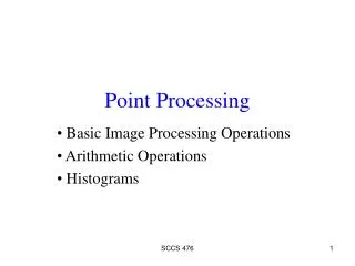
5. Homogeneous Point Processing. 3 가지 image processing operations * in A simplified approach to image processing , by Randy Crane. Point processing Modifies a pixel’s value based on that pixel’s original value or position Chapter 4 Area processing

E N D
5. Homogeneous Point Processing • 3가지 image processing operations * in A simplified approach to image processing, by Randy Crane. • Point processing • Modifies a pixel’s value based on that pixel’s original value or position • Chapter 4 • Area processing • Modifies a pixel’s value based on its original value and the values of neighboring pixels • Chapters 8-11 • Geometric processing • Changes the position or arrangement of the pixels • Chapters 14 • Frame processing • Generates pixle values based on operations on two or more images
Homogeneous point processing • Image quality (qualitative) 용어들 • washed out (smeared, blurred) • brighter • Contrast • …. • Processing 목적 • Noise suppression • Enhancement 등
Histograms • Histogram • Color image matching & retrieval 응용 • Pixel value reduction 등의 많은 응용 • PMF(Probability Mass Function) • 식 4.1 ~ 4.3 • 예) 0~255사이 값을 갖는 64개 pixel • 0값 32개, 128값 16개, 255값 16개 pixels • Histogram in Figure 4-1 ValuePMF 0 32/64 128 16/64 255 16/64
Histograms • Histogram • CMF (Cumulative Mass Function) • 식 4.6 • 예) • Histogram in Figure 4-2 ValuePMFCMF 0 32/64 0.5 128 16/64 0.75 255 16/64 1.0 • Histogram modification • CMF를 lookup table로 사용하여 PMF 변경 • Image enhancement 응용
Histogram class • Histogram class • In gui package • RGB (24 bits/pixel) image • 총 224 16 million color values • PMF is too sparse • 그래서 RGB 각각에 대한 histogram (each with 256 equal bins) • 예) figure 4.3 // histogram computation histArray = new double[256]; for(int i=0; i<width; i++) for(int j=0; j<height; j++) histArray[plane[i][j] & 0xFF]++;
Homogeneous point processing functions • Point operation • vij’ = fij(vij) • Homogeneous point operation • vij’ = f(vij) • Independent of pixel location • Linear map • f(vij) = vij • No change • Figure 4-4 • Negative image • f(vij) = 255 – vij • Figure 4-5
Using the pow function to brighten or darken • Power function • f(vij) = 255 * ( vij/255)pow • For pow<1.0, brightening but loss of contrast • 예) pow=0.9 • Figure 4-6 • 7번 적용 후 bright but washed out • For pow>1.0, darkening • 예) pow=1.5 • Figure 4-7 & 4-8 • Darkened • Histogram shifted to the left and narrowed: Figure 4-9
Using linear transforms to alter brightness and contrast • Linear transform • Linear brightness and contrast adjustment • vij’ = c*vij + b • c=contrast • b=brightness • 예) c=2, b=-90 • Figure 4-10 • 범위 넘는 값은 0과 255로 clipping
Using linear transforms to alter brightness and contrast • Display의 dynamic range에 따른 조정 • D = Dmax – Dmin • Dmax=maximum value that can be displayed • Dmin=minimum value that can be displayed • V = Vmax – Vmin • Vmax=maximum value in the image • Vmin=minimum value in the image • Linear transform 수식 • vij’ = c*vij + b • c= D / V • b=(Dmin*Vmax – Dmax*Vmin) / V
Using linear transforms to alter brightness and contrast • Display의 dynamic range에 따른 조정 • 예 • Dmin=0, Dmax=255 • Vmin=10, Vmax=90 • vij’ = (255/80)*vij – 2550/80 = 3.19*vij – 31.9 • Figure 4-11 • Applying결과: Figure 4-13 • Histogram being spread out • Contrast enhancement • lut (lookup table) 사용한 구현 • public short linearMap(short v, double c, double c) • public void linearTransform(double c, double br)
Histogram Modification • Histogram stretch • Histogram shrink • Histogram slide • Histogram equalization • ….. shrunk original stretched shifted
4.2.3 The Uniform Non-adaptive Histogram Equalization (UNAHE) • Clustering of pixel values low-contrast images, so image details 잘 보이지 않음 • Histogram equalization • Histogram modification에서 가장 보편적인 기법 • Image contrast 개선 목적
The Uniform Non-adaptive Histogram Equalization • UNAHE • Create a uniform PMF from an image that has a non-uniform PMF • Using a scaled version of the CMF as a lookup table • CMF given by Pv(a) = i=0,a pv(i) =p(V<=i) a [0..K-1] • The goal • Finding a function vij’ = f(vij) having a uniform PMF • UNAHE algorithm • vij’ = f(vij) = V*Pv(vij) • Pv(vij) : CMF • V = Vmax - Vmin • Vmax=maximum value in the image • Vmin=minimum value in the image
The Uniform Non-adaptive Histogram Equalization • UNAHE 적용 예 • 3 bits/pixel (Vmax=7, Vmin=0, V=7) • 4*4 image 3324 3566 2356 2366 • vij PMF Pv(vij) 0 0 0 1 0 0 2 3/16 3/16 3 5/16 8/16 4 1/16 9/16 5 2/16 11/16 6 5/16 16/16 7 0 16/16
The Uniform Non-adaptive Histogram Equalization • UNAHE 적용 예 • f(vij) = 7*Pv(vij) f(0) = 7*0 = 0 0 f(1) = 7*0 = 0 0 f(2) = 7*(3/16) = 1.31 1 f(3) = 7*(8/16) = 3.5 4 f(4) = 7*(9/16) = 3.93 4 f(5) = 7*(11/16) = 4.81 5 f(6) = 7*(16/16) = 7 7 f(7) = 7*(16/16) = 7 7 • 영상에 적용 4414 4577 1457 1477
The Uniform Non-adaptive Histogram Equalization • Effect of UNAHE • Figure 4.14: original & UNAHE 적용 • Figure 4.15: histograms of original and UNAHE • Figure 4.16: UNAHE and linear transform • UNAHE 적용 영상이 much higher contrast • Higher quality ?? • Low-contrast detail enhancement, but increase the contrast of noise
4.2.5 Adaptive Histogram Equalization • 지역별로 다른 특성을 갖는 영상 • 특히, document 영상 • AUHE (Adaptive Uniform Histogram Equalization) • 영상을 여러 개의 부 영상으로 분할 • 각각 부 영상에 대해 uniform histogram equalization 적용 • Fine-grained vs. coarse-grained subdivision • 적용 예 • Figure 4.22 & 4.23 • Artifact 발생 • Figure 4.24 • How to solve this problem ??