Download
1 / 10
110 likes | 382 Vues
Alternation and Polynomial Time Hierarchy. Alternating Turing Machine (ATM) node is marked accept iff any of its children is marked accept . node is marked accept iff all of its children are marked accept . .

E N D
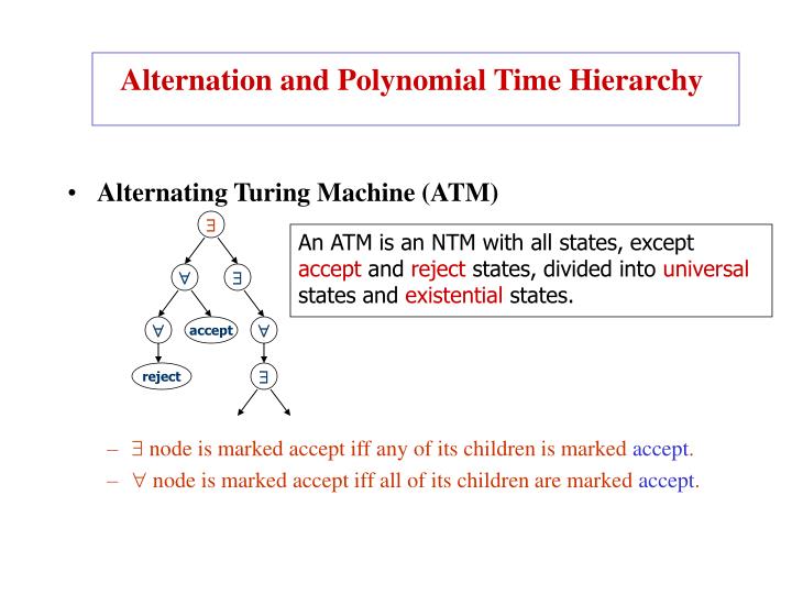
Alternation and Polynomial Time Hierarchy • Alternating Turing Machine (ATM) • node is marked accept iff any of its children is marked accept. • node is marked accept iff all of its children are marked accept. An ATM is an NTM with all states, except accept and reject states, divided into universalstates and existential states. accept reject
Alternating Time and Space : ATIME(f(n))={ L : an ATM that accepts L and use O(f(n)) time on all branches } ASPACE(f(n)) is defined similarly. AL= ASPACE(log n), AP = ATIME(nk) . • eg. MIN-FORMULA={ < > | is a minimal Boolean formula, i.e., there is no shorter equivalent}.
MIN-FORMULAAP. On input : 1. Universally select all formula f that are shorter than . 2. Existentially select an assignment to the input variables of . 3. Evaluate both and f on this assignment. 4. Accept if the formulas evaluate to different values; else reject. • Thm: ATIME(f(n)) SPACE(f(n)) ATIME(f2(n)) . Thus, AP = PSPACE . • Thm: ASPACE(f(n)) = TIME(2O(f(n))) . Thus, ASPACE = EXP .
Lemma: For f(n) >= n we have ATIME(f(n)) SPACE(f(n)). Proof: Convert an O(f(n))-time ATM M to a O(f(n))-space DTM S. S makes a depth-first search of M’s computation tree to determine whether the start configuration is “accept” or not. It is done by recursion and the depth is O(f(n)), since the computation tree has depth O(f(n)). For each level of recursion, the stack store the non-det choice that M made to reach that configuration from its parent and this uses only constant space. S can recover the configuration by “replaying” the computationfrom the start and following the recorded “signposts.”
Lemma: Let f(n)>= n we have SPACE(f(n)) ATIME(f2(n)). • Proof: • Let M be an O(f(n))-space DTM. We want to construct an • O(f2(n))-time ATM S to simulate M. • It is very similar to the proof of Savitch’s Theorem. • c1,c2,t=m [c1,m, t/2 m,c2,t/2 ]: indicate if C2 is reachable • from C1 in t steps for M. • S uses the above recursive alternating procedure to test whether the start configuration can reach an accepting conf. within 2df(n) steps. The recursive depth is O(f(n)). • For each level it takes O(f(n)) time to write a conf. (why?) • Thus the algorithm runs in O(f2(n)) alternating time.
Lemma: f(n) >= log n we have ASPACE(f(n)) TIME (2O(f(n))) . • Proof: • Construct a 2O(f(n)) -time DTM S to simulate an O(f(n))-space • ATM M. On input w, S constructs the following graphs of the computation M on w. • Nodes are conf of M on w and edges go from a conf to those configurations that it can yield in a step. • After the graph is constructed, S repeatedly scans it and marks certain conf as accepting. Initially, only actual accepting conf are marked “accepting”. A conf that performs universal branching is marked “accepting” if all its children are marked and an existential conf is marked if any of its children are marked. • S continues until no additional nodes are marked in a scan. Finally, S checks if the start conf is marked. There are 2O(f(n)) conf of M on w, which is also the size of the graph. Hence the total time used is 2O(f(n)) .
Lemma: f(n) >= log n we have ASPACE(f(n)) TIME (2O(f(n))) . Proof: Construct an O(f(n))-space ATM S to simulate a 2O(f(n)) -time DTM M. On input w, S has only enough space to store pointers into a tableau of the computation M on w as depicted in the following. The content of d is determined by the contents of its parents a, b, and c. # q0 w1 # start configuration cell # # 2nd configuration # # window a b c d # # th configuration
S operates recursively to guess and then verify the contents of the individual cells of the tableau. It is easy to verify the cells of the first row, since it knows the start conf of M on w. For other cell d, S existentially guesses the contents of the parents, checks whether their contents would yield d’s contents according to M’s transition, and then universally branches to verify these guesses recursively. Assume M moves its head to the leftmost cell after entering accepting state. Thus S can determine whether M accepts w by checking the contents of the lower leftmost cell of the tableau. Hence S never needs to store more than a pointer to a cell in the tableau. So it uses at most O(f(n)) space.
Polynomial Hierarchy: Let kT(n) be a class of language L accepted by an Alternating Turing Machine that begins in an existential state, alternates between and states k-1 times and halts within O(T(n)) . • Define The class of complement of languages within kP is called kP = co-kP. kP: where ATM begins in a state. Note that kP k+1P and kP k+1P , 1P=NP and 1P=co-NP . MIN-CIRCUIT is in 2P.
Def: The polynomial hierarchy • Thm: If kPkP for some k1 ,then PNP . • Prop: If there exists a language L that is complete for PH, then there exists k s,t, the hierarchy collapses to level k .