Download

1 / 32
320 likes | 461 Vues
Finite mixture modeling. BST 764 – Fall 2014 – Dr. CHARNIGO – Unit THREE. Contents: Formulation… 3-8 Parameter estimation… 9-13 Likelihood ratio testing… 14-16 Modified likelihood ratio testing … 17-18 D testing… 19-24 Practical applications… 25-32. Formulation.

E N D
Finite mixture modeling BST 764 – Fall 2014 – Dr. CHARNIGO – Unit THREE
Contents:Formulation… 3-8Parameter estimation… 9-13Likelihood ratio testing… 14-16Modified likelihood ratio testing … 17-18D testing… 19-24Practical applications… 25-32
Formulation Have a look at the following graphs: Figure 1
Formulation Figure 2
Formulation Figure 3
Formulation The histogram in Figure 1 exhibits a clear bimodal pattern. A commonly encountered parametric distribution will not suffice to describe it. The histogram in Figure 2 does not exhibit a clear bimodal pattern, but bell-shaped may not be an apt description; the middle is too “fat”. Again, a commonly encountered parametric distribution will not suffice. The histogram in Figure 3 looks bell-shaped, and if we weren’t alerted to the contrary we would probably try to describe it using a normal distribution.
Formulation All three figures in fact display data from what we call finite mixture models, more specifically two-component normal mixture models. We can describe them as follows: Let X be Bernoulli with parameter 1/2. Given that X = x, let Y have a conditional normal distribution with mean μx and standard deviation 1. In Figures 1, 2, and 3 I took μ equal to 4, 2, and 1 respectively. Then the marginal distribution of Y is a two-component normal mixture.
Formulation More generally, we can take X to be a discrete random variable with finite support {0, 1, 2, …, J – 1}. Define px := P(X = x). Given that X = x, we can take Y to have the conditional probability density function f(y; θx), where f is from a known parametric family and θxis a vector of parameters. Then the marginal distribution of Y is a finite mixture. In the preceding example we had J = 2, p0 = p1 = 1/2, f from the family of normal distributions, θ0 = (0, 1)T, and θ1 = (µ, 1)T. Problem: Show by examples that a three-component normal mixture can have three modes, two modes, or close to a bell-shaped appearance. Show by another example that a three-component normal mixture can appear somewhat like a skewed parametric distribution (e.g., gamma).
Parameter Estimation If we knew J and could observe both X and Y, then parameter estimation would be straightforward; for instance, we might employ maximum likelihood. If we knew J and could observe only Y but not X, then parameter estimation could be accomplished, in principle, using maximum likelihood. However, because such a likelihood function would be complicated, an approach such as expectation maximization is more commonly employed (more on that in the next slides). If we don’t know J, then we need to employ some inferential procedure to guess what J may be. Once we’ve made our guess (more on that later), we can use expectation maximization as above.
Parameter Estimation To motivate expectation maximizationRef1, suppose that we could observe X. Then the “complete data log likelihood function” would be ∑i=1n ∑x=0J-1 I(Xi = x) {log px + log f( Yi ; θx )}. If we can’t observe X, we may consider replacing I(Xi = x) by its expected value given Yi = y, which is P(Xi = x | Yi = y). Exercise: Show that P(Xi = x | Yi = y) = px f(y; θx) / ∑m=0J-1 pm f(y; θm). (Since Yi = y is a zero-probability event, condition on y-δ< Yi< y+δ for small δ and then let δ→0.) Exercise: What is problematic about replacing I(Xi = x) by P(Xi = x | Yi = y) ? Ref1. Dempster, A.P., Laird, N.M., and Rubin, D.B. (1977). Maximum likelihood from incomplete data via the EM algorithm. J. R. Statist. Soc. B, 39, 1-22.
Parameter Estimation Suppose that we have “initial values” for the unknown parameters. Call them px(0) and θx(0). Then we can estimate P(Xi = x | Yi = y) as px(0)f(y; θx(0)) / ∑m=0J-1pm(0)f(y; θm(0)) and maximize ∑i=1n ∑x=0J-1px(0)f(Yi; θx(0)) / ∑m=0J-1 pm(0)f(Yi; θm(0)){log px + log f( Yi ; θx)} with respect to px and θx. The results are called px(1)and θx(1). Then we can maximize ∑i=1n ∑x=0J-1px(1)f(Yi; θx(1)) / ∑m=0J-1pm(1)f(Yi; θm(1)) {log px + log f( Yi ; θx)}.
Parameter Estimation The results of the latter maximization are called px(2)and θx(2). We continue this process iteratively, obtaining px(t) and θx(t) for t = 3, 4, … until some stopping criterion is satisfied. At that juncture, we consider ourselves to have estimated pxand θx. Exercise: What sort of stopping criterion might be considered ? Exercise: Why do you suppose this was called the expectation maximization algorithm ?
Parameter Estimation Expectation maximization is intended to provide an approximation to maximum likelihood, and each iteration does in fact increase the likelihood. Thus, while one is not guaranteed to end up with a satisfactory answer (i.e., a global maximizer rather than a local maximizer), one will obtain a better answer than one’s initial values. Exercise: Under what circumstances do you think expectation maximization may be sensitive to initial values ? How might you cope with sensitivity to initial values ? Under some circumstancesRef2, the maximum likelihood estimators (which are approximated by expectation maximization) will be n1/2-consistent. To avoid confusion later, note that n1/2-consistency assumes knowledge of J. Ref2. Redner, R.A. and Walker, H.F. (1984). Mixture densities, maximum likelihood, and the EM algorithm. SIAM Review, 26, 195-239.
Likelihood ratio testing Consider the problem of testing H0: J = 1 against H1: J = 2 when the model parameters are unknown. This is a homogeneity test. Using notation from the two-component model, the null hypothesis may be expressed as (θ1 – θ0) p0 p1 = 0. Since model parameters are not identifiable when the null hypothesis is true (i.e., their values are not uniquely determined), the usual regularity conditions for likelihood ratio testing are not satisfied. In fact, negative twice the log likelihood ratio test statistic does not have an asymptotic chi-square distribution when the null hypothesis is trueRef3. Ref3 Ghosh, J.K. and Sen, P.K. (1985). On the asymptotic performance of the log likelihood ratio statistics for the mixture model and related results. In Proceedings of the Berkeley Conference in Honor of J. Neyman and J. Kiefer (Lucien M. Le Cam and Richard A. Olshen, eds.) 2, 789-806.Wadsworth.
Likelihood ratio testing Still, a likelihood ratio test is possible. If J = 1, then the model may be simplified to f(y; θnull). Letting an asterisk denote maximum likelihood estimation (in practice, approximated by expectation maximization under the alternative hypothesis), the test statistic is -2 ∑i=1n log f(Yi; θnull*) + 2 ∑i=1nlog{ p0* f(Yi; θ0*) + p1* f(Yi; θ1*) }. When the null hypothesis is true and certain conditions are satisfied (including that θis a scalar or only one component of the vector is unknown)Ref4, the aforementioned quantity converges in law to sup(θin Θ) { max(W(θ), 0) }2, with W(θ) a Gaussian process and Θthe compact parameter space. Ref4 Chen, H. and Chen, J. (2001). The likelihood ratio test for homogeneity in the finite mixture models. Canadian Journal of Statistics, 29, 201-215.
Likelihood ratio testing The quantiles of sup(θ in Θ) { max(W(θ), 0) }2 cannot be found in a chi-square (or any other commonly available) table. They can be estimated by simulation Ref5 or approximated by random field theoryRef6. Exercise: Other than the work, what is undesirable about this situation ? Ref5 McLachlan, G. (1987). On bootstrapping the likelihood ratio test statistic for the number of components in a normal mixture. Appl. Statist., 36, 318-324. Ref6Sun, J. (1993). Tail probabilities of the maxima of Gaussian random fields. Ann. Probab. 21, 34-71. Let us now discuss Ref5 and Ref4.
Modified likelihood ratio testing Suppose now that θ is a scalar. Chen, Chen, and KalbfleischRef7suggested modifying the log likelihood function by adding a penalty, ∑i=1n log{ p0f(Yi; θ0) + p1 f(Yi ; θ1) } + C log{ 4 p0 p1 }, where C is a positive constant. Call this L(p0,p1,θ0,θ1). Exercise: Can you interpret the penalty as a prior distribution in a Bayesian framework ? How do you think that the penalty affects estimation ? The modified likelihood ratio test statistic is defined as 2 L(p0*, p1*, θ0*, θ1*) – 2 L(1/2, 1/2, θnull*, θnull*). Ref7Chen, H., Chen, J., and Kalbfleisch, J. (2001). A modified likelihood ratio test for homogeneity in finite mixture models. J. R. Statist. Soc. B, 63, 19.
Modified likelihood ratio testing When the null hypothesis is true and certain conditions are satisfied, the test statistic converges in law to { max(W(θnull), 0) }2. Exercise: Can this be related to a chi-square distribution ? Exercise: The asymptotic conclusion does not depend on the chosen value of C. In practice, how might one choose C ? Exercise: What inferential tasks appear to be left unresolved by the modified likelihood ratio test ? Let us now discuss Ref7.
D testing One weakness of the modified likelihood ratio test is that the test statistic cannot be calculated without the individual values of Y1, Y2, …, Yn. While hoping to calculate a test statistic without the individual values of the response variable seems fanciful, consider the following scenario. Year 1. We obtain Y1, Y2, …, Y10000. We estimate parameters and calculate a test statistic. We then discard Y1, Y2, …, Y10000. Year 2. We obtain Y10001, Y10002, …, Y20000. We want to re-estimate parameters and re-calculate the test statistic. We saved the parameter estimates and test statistic from last year, but do we also need to retrieve the individual values of Y1, Y2, …, Y10000 to proceed ?
D testing In some simple problems, at least, the answer is no. For example, to estimate E[Y1] in Year 1, one may compute a sample mean based on Y1 through Y10000. To estimate E[Y1] in Year 2, one may compute a sample mean based on Y10001 through Y20000 and then simply average the two sample means; recalling Y1 through Y10000 themselves is unnecessary ! While I was not aware of such updating formulas for mixture model parameter estimation, my Ph.D. advisor seemed to recognize the possibility that they might someday be developed, and she did later work on that. Anyway, this possibility motivated the D test.
D testing The basic idea was to define a test statistic that depended on Y1, Y2, …, Yn only through the estimators of p0, p1, θ0, θ1, and θnull. (A loose analogy can be made to the concept of a sufficient statistic, which some of you have studied.) More specifically, the test statistic was defined to be the (squared) L2 distance between fitted homogeneous and heterogeneous models, dn := ∫ | f(x; θnull*) – p0* f(x; θ0*) – p1* f(x; θ1*) |2 dx. Exercise: Why use L2 distance instead of L1 distance ?
D testing Under some conditions, weRef8 found that dn = Op(n-1) if the null hypothesis was true. Since dn converges in probability to a nonzero constant if the null hypothesis is false, this implies that a test based on dn can distinguish between the null and alternative hypotheses if an appropriate critical value is found. (Why ?) Such a critical value could be estimated by simulation, but that could make the D test far less practical than the modified likelihood ratio test. Ref8Charnigo, R. and Sun, J. (2004). Testing homogeneity in a mixture distribution via the L2 distance between competing models. Journal of the American Statistical Association, 99, 488.
D testing Later, weRef9 identified an appropriate critical value for the D test based on asymptotic theory. In fact, if the null hypothesis was true, then K n dn= ( max{0, ∑i=1n Wi } )2 / ∑i=1n Wi 2 + op(1), where K is estimable and Wi is a function of Yi with E[W1]=0. Exercise: If the null hypothesis was true, then K n dn converges in law to 0.5 χ20 + 0.5 χ21, the same as the modified likelihood ratio test statistic. Ref9Charnigo, R. and Sun, J. (2010). Asymptotic relationships between the D-test and likelihood ratio-type tests for homogeneity. StatisticaSinica, 20, 497.
D testing Exercise: Why not make ( max{0, ∑i=1n Wi } )2 / ∑i=1n Wi 2 itself the test statistic, which is much simpler than either the D test or the modified likelihood ratio test ? Problem: Using the data from Figure 1 (see R code below), perform the D test for a normal mixture using an expectation maximization approximation to penalized maximum likelihood with C = 1 and quoting without proof the result that K = π1/2 (16/3). Repeat for the data from Figure 2 and Figure 3 (replace 4*x by 2*x and x in the R code below). set.seed(102) x <- sort(( runif(1000) > 0.5 ) + 0) y <- rnorm(1000) + 4*x Let us discuss Ref8 and Ref9.
Practical applications In the papers examined so far, we have seen (or heard of) some practical applications of finite mixture modeling: • Quantifying agricultural yield • Describing crab morphometry • Establishing heterogeneity in blood chemistry • Measuring firms’ financial performances
Practical applications We shall now consider two more practical applications. The first is to microarray data analysis. Expression levels are measured for many genes (hundreds or thousands), for each of several persons with a medical condition and each of several persons without (perhaps a dozen persons or so in total). For each gene, a two-sample T test (or some variant thereof) is performed to compare the mean expression level for persons with the medical condition to that for persons without.
Practical applications So, one obtains hundreds or thousands of T test statistics. Each of these may be converted to a Z score or a P value. Exercise: How can a T score be converted to a Z score ? Exercise: What information may be lost if a T score is converted to a P value ? Exercise: What is the problem with conducting hundreds or thousands of T test statistics ? What are some “traditional” approaches to dealing with this problem, and what may be their limitations ?
Practical applications My former Ph.D. student Hongying Dai and I developed methodologyRef10to test the null hypothesis that P values were uniformly distributed versus the alternative hypothesis that they arose from a mixture of a uniform distribution and a beta distribution. This methodology could be incorporated into a filtration algorithm, providing an alternative to “traditional” approaches to addressing the aforementioned problem. Ref10 Dai, H. and Charnigo, R. (2008). Omnibus testing and gene filtration in microarray data analysis. Journal of Applied Statistics, 35, 31.
Practical applications We also developed methodologyRef11to test the null hypothesis that Z scores came from a zero-mean normal distribution (variance unknown) versus the alternative hypothesis that they arose from a mixture of zero-mean and nonzero-mean normal distributions (variance unknown). This methodology, too, could be incorporated into a filtration algorithm. Let us now discuss Ref10 and Ref11. Ref11 Dai, H. and Charnigo, R. (2010). Contaminated normal modeling with application to microarray data analysis. Canadian Journal of Statistics, 38, 315.
Practical applications The second additional practical application is to birthweight data. Superficially, a normal distribution may appear to provide a good fit to birthweight data. However, the left tail and, to a lesser degree, the right tail may be thicker than would be consistent with a normal distribution. Since the left tail and right tail are where the risks of mortality and morbidities may be elevated, describing these portions of the distribution more accurately may be relevant to seeking additional insight into the relationships among birthweight, mortality, and morbidities.
Practical applications Lorie Chesnut, Tony LoBianco, and I proposed modeling birthweight distribution as a mixture of a finite but unspecified number of normal distributions.Ref12 We presented an information-type criterion based on previous unpublished workRef13that could help select the number of components. Since there was no explicit hypothesis testing per se, there was no need to worry about finding an asymptotic null distribution and critical values for a test statistic. Ref12Charnigo, R., Chesnut, L.W., LoBianco, T., and Kirby R.S. (2010). Thinking outside the curve, Part I: Modeling birthweight distribution. Biomedcentral Pregnancy and Childbirth, 10, Article 37. Ref13Pilla, R. S. and Charnigo R. Consistent estimation and model selection in semiparametric mixtures. Unpublished manuscript.
Practical applications Exercise: Argue for and against treating within-component variances as equal. Exercise: Even though no critical values were required, extensive simulation studies were conducted. Why ? As suggested by previous authors who had considered two-component mixture models (e.g., Ref14), a possible interpretation is that one component represents “normal” births while the rest of the model represents “compromised” births. Ref14Gage, T., Bauer, M., Heffner, N., and Stratton, H. (2004). Pediatric paradox: heterogeneity in the birth cohort. Human Biology, 76, 327–342. Let us discuss Ref12 and Ref13.