Download
1 / 107
1.07k likes | 1.18k Vues
Petri Nets ee249 Fall 2000. Marco Sgroi Most slides borrowed from Luciano Lavagno’s lecture ee249 (1998). Models Of Computation for reactive systems. Main MOCs: Communicating Finite State Machines Dataflow Process Networks Discrete Event Codesign Finite State Machines Petri Nets

E N D
Petri Netsee249 Fall 2000 Marco Sgroi Most slides borrowed from Luciano Lavagno’s lecture ee249 (1998)
Models Of Computationfor reactive systems • Main MOCs: • Communicating Finite State Machines • Dataflow Process Networks • Discrete Event • Codesign Finite State Machines • Petri Nets • Main languages: • StateCharts • Esterel • Dataflow networks
Outline • Petri nets • Introduction • Examples • Properties • Analysis techniques • Scheduling
Petri Nets (PNs) • Model introduced by C.A. Petri in 1962 • Ph.D. Thesis: “Communication with Automata” • Applications: distributed computing, manufacturing, control, communication networks, transportation… • PNs describe explicitly and graphically: • sequencing/causality • conflict/non-deterministic choice • concurrency • Asynchronous model (partial ordering) • Main drawback: no hierarchy
Petri Net Graph • Bipartite weighted directed graph: • Places: circles • Transitions: bars or boxes • Arcs: arrows labeled with weights • Tokens: black dots p2 t2 2 t1 p1 p4 3 t3 p3
Petri Net • A PN (N,M0) is a Petri Net Graph N • places: represent distributed state by holding tokens • marking (state) M is an n-vector (m1,m2,m3…), where mi is the non-negative number of tokens in place pi. • initial marking (M0) is initial state • transitions: represent actions/events • enabled transition: enough tokens in predecessors • firing transition: modifies marking • …and an initial marking M0. p2 t2 2 t1 p1 p4 3 Places/Transition: conditions/events t3 p3
Transition firing rule • A marking is changed according to the following rules: • A transition is enabled if there are enough tokens in each input place • An enabled transition may or may not fire • The firing of a transition modifies marking by consuming tokens from the input places and producing tokens in the output places 2 2 2 2 3 3
Concurrency, causality, choice t1 t2 t5 t3 t4 t6
Concurrency, causality, choice t1 Concurrency t2 t5 t3 t4 t6
Concurrency, causality, choice t1 t2 t5 Causality, sequencing t3 t4 t6
Concurrency, causality, choice t1 t2 t5 Choice, conflict t3 t4 t6
Concurrency, causality, choice t1 t2 t5 Choice, conflict t3 t4 t6
Confusion • t1 and t2 are concurrent but their firing order is not irrelevant for conflict resolution (not local choice) • From (1,1,0,0,0): • solving a conflict (t1,t2) (0,0,0,0,1),(0,0,1,1,0) • not solving a conflict (t2,t1) (0,0,1,1,0) p1 p3 t1 p5 t3 p4 p2 t2
Communication Protocol Send msg Receive msg P2 P1 Send Ack Receive Ack
Communication Protocol Send msg Receive msg P2 P1 Send Ack Receive Ack
Communication Protocol Send msg Receive msg P2 P1 Send Ack Receive Ack
Communication Protocol Send msg Receive msg P2 P1 Send Ack Receive Ack
Communication Protocol Send msg Receive msg P2 P1 Send Ack Receive Ack
Communication Protocol Send msg Receive msg P2 P1 Send Ack Receive Ack
Producer-Consumer Problem Produce Buffer Consume
Producer-Consumer Problem Produce Buffer Consume
Producer-Consumer Problem Produce Buffer Consume
Producer-Consumer Problem Produce Buffer Consume
Producer-Consumer Problem Produce Buffer Consume
Producer-Consumer Problem Produce Buffer Consume
Producer-Consumer Problem Produce Buffer Consume
Producer-Consumer Problem Produce Buffer Consume
Producer-Consumer Problem Produce Buffer Consume
Producer-Consumer Problem Produce Buffer Consume
Producer-Consumer Problem Produce Buffer Consume
Producer-Consumer Problem Produce Buffer Consume
Producer-Consumer Problem Produce Buffer Consume
Producer-Consumer Problem Produce Buffer Consume
Producer-Consumer Problem Produce Buffer Consume
Producer-Consumer with priority A Consumer B can consume only if buffer A is empty Inhibitor arcs B
PN properties • Behavioral: depend on the initial marking (most interesting) • Reachability • Boundedness • Schedulability • Liveness • Conservation • Structural: do not depend on the initial marking (often too restrictive) • Consistency • Structural boundedness
Reachability • Marking M is reachable from marking M0 if there exists a sequence of firingss = M0 t1 M1 t2 M2… M that transforms M0 to M. • The reachability problem is decidable. p2 t2 M0 = (1,0,1,0) t3 M1 = (1,0,0,1) t2 M = (1,1,0,0) p1 t1 p4 t3 p3 M0 = (1,0,1,0) M = (1,1,0,0)
Liveness • Liveness: from any marking any transition can become fireable • Liveness implies deadlock freedom, not viceversa Not live
Liveness • Liveness: from any marking any transition can become fireable • Liveness implies deadlock freedom, not viceversa Not live
Liveness • Liveness: from any marking any transition can become fireable • Liveness implies deadlock freedom, not viceversa Deadlock-free
Liveness • Liveness: from any marking any transition can become fireable • Liveness implies deadlock freedom, not viceversa Deadlock-free
Boundedness • Boundedness: the number of tokens in any place cannot grow indefinitely • (1-bounded also called safe) • Application: places represent buffers and registers (check there is no overflow) Unbounded
Boundedness • Boundedness: the number of tokens in any place cannot grow indefinitely • (1-bounded also called safe) • Application: places represent buffers and registers (check there is no overflow) Unbounded
Boundedness • Boundedness: the number of tokens in any place cannot grow indefinitely • (1-bounded also called safe) • Application: places represent buffers and registers (check there is no overflow) Unbounded
Boundedness • Boundedness: the number of tokens in any place cannot grow indefinitely • (1-bounded also called safe) • Application: places represent buffers and registers (check there is no overflow) Unbounded
Boundedness • Boundedness: the number of tokens in any place cannot grow indefinitely • (1-bounded also called safe) • Application: places represent buffers and registers (check there is no overflow) Unbounded
Conservation • Conservation: the total number of tokens in the net is constant Not conservative
Conservation • Conservation: the total number of tokens in the net is constant Not conservative
Conservation • Conservation: the total number of tokens in the net is constant Conservative 2 2
Analysis techniques • Structural analysis techniques • Incidence matrix • T- and S- Invariants • State Space Analysis techniques • Coverability Tree • Reachability Graph