Contribution of Ocean, Fossil Fuel, Land Biosphere and Biomass Burning

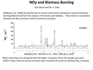
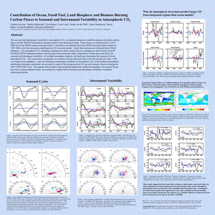
1. Why do atmospheric inversions predict larger IAV from integrated regions than ocean models? Contribution of Ocean, Fossil Fuel, Land Biosphere and Biomass Burning Carbon Fluxes to Seasonal and Interannual Variability in Atmospheric CO2 Cynthia Nevison1, Natalie Mahowald1, Scott Doney2, Ivan Lima2, Guido van der Werf3, James Randerson4, David Baker1, Prasad Kasibhatla5 and Galen McKinley6 1 National Center for Atmospheric Research, 2 Woods Hole Oceanographic Institution, 3Vrije Universitat, 4 UC, Irvine, 5 Duke University, 6 University of Wisconsin Abstract The seasonal and interannual variability in atmospheric CO2 is simulated using best available estimates of surface carbon fluxes and the MATCH atmospheric transport model with interannual winds. Ocean fluxes are obtained from a 1979-2004 run of the WHOI ocean ecosystem model. Land fluxes are obtained from the GFED terrestrial carbon model for 1997-2004, with fire emissions scaled based on CO inversion results. Fossil fuel emissions are obtained from CDIAC databases. The atmospheric CO2 variability resulting from these surface fluxes is compared to observations from 89 GLOBALVIEW monitoring stations with the goal of assessing the relative importance of land and ocean fluxes for seasonal and interannual variability. At northern hemisphere stations, the land tracer dominates the seasonal cycle in atmospheric CO2. The ocean tracer is generally out of phase with the observed total cycle and accounts for only ~10% on average of its amplitude. Land also dominates interannual variability in atmospheric CO2 in the northern hemisphere, and biomass burning in particular can account for much of the strong positive CO2 growth anomaly observed during the 1997-1998 ENSO event. The signals from northern land extend throughout the southern hemisphere, but oceanic fluxes also exert a strong influence there, accounting for roughly half of seasonal and interannual variability at southern monitoring stations. Figure 5. Interannual variability in integrated surface fluxes. Blue line is WHOI ocean model, red line is MIT ocean model. Black line is the IAV in ocean fluxes inferred by the Transcom3 atmospheric CO2 inversion [Baker et al., 2006]. Regions are defined based on aggregated Transcom3 regions. Interannual Variability Seasonal Cycles Experiment: Impose Baker et al. [2006] monthly IAV on spatially uniform surface CO2 fluxes from 11 Transcom regions. Run in MATCH atmospheric transport model. Compare IAV in atmospheric CO2 to MATCH run with WHOI ocean model fluxes. Figure 6. Root mean square variability in surface ocean CO2 fluxes from 1988-2003, a) WHOI ocean model, b) Experimental “Transcom” fluxes. Shows that the magnitude of RMS variability in the surface fluxes is locally smaller for “Transcom” than WHOI at most extratropical gridpoints, but, unlike WHOI, “Transcom” fluxes are spatially and temporally coherent within each region. Figure 3. Atmospheric CO2 growth rate anomalies at 6 selected stations. Thin black line with symbols is GLOBALVIEW observations, blue line is WHOI ocean, green line is net GFED land, red line is biomass burning, magenta line is fossil fuel. Solid heavy black line is model best case total CO2. a) BRW, b) NWR, c) MLO, d) SMO, e) CGO, f) PSA. Figure 1. Seasonal cycles of atmospheric CO2 at 6 selected stations. Thin black line with triangles is GLOBALVIEW observed cycle. Blue line is WHOI ocean, cyan line is Takahashi et al.[2002] ocean. Green line is net GFED land, red line is biomass burning. Magenta line is fossil fuel. Heavy black line is total CO2. a) Barrow, Alaska, b) Niwot Ridge, Colorado, c) Mauna Loa, Hawaii, c) Samoa, e) Cape Grim, Tasmania, f) Palmer Station, Antarctica. Figure 7. Interannual variability in WHOI and “Transcom” atmospheric CO2 tracers at 6 stations. Shows that the WHOI and Transcom tracers have similar atmospheric variability, despite the fact that the integrated Transcom fluxes are 2-5 times larger within broad ocean regions (Figure 5). These results suggest that local ocean flux variations, which largely cancel each other out when integrated over broad regions, interact with transport near remote atmospheric measurement sites to create part of the variability observed at these sites. Atmospheric inversions may translate these signals into overly large variability in the surrounding large ocean regions because the flux patterns (e.g., spatially uniform in Transcom) used in the inversions do not account for local flux variability. Figure 2. Taylor diagrams comparing the model seasonal cycle in total or component CO2 tracers to GLOBALVIEW observations at 89 stations. Each symbol represents a different station. The angle  from the x-axis is the arccos of the correlation coefficient R between the model and observed cycle, which reflects the agreement in phasing. The radial axis value is the ratio of standard deviations: model/obs, which represents the agreement in amplitude. Red triangles are extratropical (> 25°N) NH stations, magenta circles are tropical NH stations, cyan circles are tropical SH stations, blue triangles are extratropical (< -25°S) SH stations. The stations featured in Figure 1 are explicitly labeled with their 3-letter code. a) total CO2, b) total CO2 NH stations only, c) WHOI ocean, d) net GFED land Figure 4. Taylor diagrams comparing IAV in model total and component CO2 tracer growth rate anomalies to GLOBALVIEW observations. See Figure 2 for explanation of Taylor diagrams and symbols. a) total CO2, b) net GFED land (=BB+NEP), c) biomass burning (BB), d) Net ecosystem production (NEP), e) WHOI ocean, f) fossil fuel. Figures a-d include 89 stations from 1997-2004. Figures e-f include 33 stations from 1979-2004. • Baker, D. F., et al., TransCom 3 inversion intercomparison: Impact of transport model errors on the interannual variability of regional CO2 fluxes, 1988–2003, Global Biogeochem. Cycles, 20, 2006. • Acknowledgements:We acknowledge the support of NASA grant NNG05GG30G and NSF grant ATM0628472. We also thank the many contributors to the GLOBALVIEW data products.