Download

1 / 85
850 likes | 959 Vues
Finance 30210: Managerial Economics. Consumer Demand Analysis. We can begin our representation of the consumer with a demand function…. Is a function of…. Quantity demanded. Price. Income. Prices of Compliments. Prices of Substitutes. Price. $20. Quantity. 40.

E N D
Finance 30210: Managerial Economics Consumer Demand Analysis
We can begin our representation of the consumer with a demand function… Is a function of… Quantity demanded Price Income Prices of Compliments Prices of Substitutes Price $20 Quantity 40
Given a demand function we can characterize the behavior of demand with elasticity.. Price Price elasticity will always be a negative number $20 $15 Quantity 40 60
Given a demand function we can characterize the behavior of demand with elasticity.. Income elasticity will generally be a positive number Price $20 Quantity 40 56
Given a demand function we can characterize the behavior of demand with elasticity.. Cross price elasticity will be a positive number for substitutes Price $20 Quantity 40 44
Given a demand function we can characterize the behavior of demand with elasticity.. Cross price elasticity will be a negative number for compliments Price $20 Quantity 32 40
Note that if the demand relationship is linear, elasticity is not constant
For example…. Price $80 $30 Quantity 100
Let’s try something a little more complicated…a non-linear demand relationship Price $2916 $400 Quantity 68
Sometimes we use demand functions that are linear in logs… Price Price $12 $12 Quantity LN(Quantity) 40 3.7
Price $12 Quantity 40
A little math trick…recall the derivative of the natural log This just says that the difference in logs is a percentage change Therefore, if we start with elasticity
Sometimes we use demand functions that are linear in logs… Price $12 LN(Quantity) 3.7
Sometimes we use demand functions that are linear in logs… Price LN(Price) $10 2.3 Quantity Quantity 3 3
Sometimes we use demand functions that are linear in logs… LN(Price) 2.3 Quantity 3
Sometimes we use demand functions that are linear in logs… Price LN(Price) $5 1.6 Quantity LN(Quantity) 8.8 2.2
Sometimes we use demand functions that are linear in logs… LN(Price) 1.6 Log linear demand curves have constant elasticities! LN(Quantity) 2.2
Suppose that you setting prices for US Air. You know that you face the following demand curve for the New York/Chicago Shuttle… Price $200 $80,000 If you wanted to increase revenues, should you increase or decrease your price? Quantity 400
If you wanted to increase revenues, should you increase or decrease your price? Price Why didn’t revenue go up by $400? $200 $199 $80,396 Quantity 400 404 You should decrease price. A $1 price decrease will raise revenues by $400
Suppose that you wanted to maximize revenues? Price $200 $150 $90,000 Quantity 400 600
Now, let’s go about this a little differently… Price $200 $80,000 Every 1% drop in price will raise revenues by 1% Quantity 400
Using the point elasticity gives you the same answer… Why didn’t revenues go up by 10%? Price $200 $180 $86,400 Quantity 400 480
We could also maximize revenues using elasticity… When the elasticity hits -1, revenues stop growing when you lower your price. Price $150 $90,000 Quantity 600
Obviously, the more information you have, the better decisions you will make… However, knowing a few elasticities is quite helpful as well! The best pricing decisions would come from a demand curve Price Price Revenue maximizing price Revenue maximizing price $250 $200 $150 $140 $90,000 $50 Quantity Quantity 600 600
Suppose that you setting prices for US Air. You know that you face the following demand curve for the New York/Chicago Shuttle… Suppose that median income is equal to $50,000. Income in thousands Price Suppose that a recession causes a 20% drop in income. How much would we have to lower our price if we wanted to keep sales constant? $125 $75,000 Quantity 600
Suppose that a recession causes a 20% drop in income. How much would we have to lower our price if we wanted to keep sales constant? Now income is $40,000 Price $125 $120 $72,000 Quantity 600
Now, again with elasticity… Suppose that median income is equal to $50,000. Price $125 Suppose that a recession causes a 20% drop in income. How much would we have to lower our price if we wanted to keep sales constant? $75,000 Quantity 600
Suppose that a recession causes a 20% drop in income. How much would we have to lower our price if we wanted to keep sales constant? Price $125 $123 $73,800 Quantity 600
Again, the more information you have, the better decisions you will make… However, knowing a few elasticities is quite helpful as well! The best pricing decisions would come from a demand curve Price Price $125 $125 $75,000 $75,000 Quantity Quantity 600 600
Now, suppose that you realized that you actually faced two types of customers : Recreational and business travelers. Could you do better? Business Recreational Price Price $400 $200 $150 $150 $75,000 $15,000 Quantity Quantity 500 100
Recall the aggregate demand curve we had previously….what we had was actually a piece of what aggregate demand really looked like Price At a price above $200, recreational travelers don’t fly. The only demand is coming from business travelers. $400 At a price below $200, we now have two types of demanders flying. $200 + $150 $90,000 Could we do better? Quantity 400 600
Suppose that we decided to ignore recreational travelers and cater to business clients… Price $400 $200 $80,000 No…that’s not a good idea! Quantity 400 600
Why don’t we just charge them different prices? Recreational Business Price Price $400 $200 $200 $100 $80,000 $20,000 Quantity Quantity 400 200
The real question is: Is this feasible to do empirically? Price $400 This is “the Truth”. Two types of individuals making purchasing decisions. Individual decisions added up across all individuals create an aggregate demand curve. $200 Quantity
If you do a linear estimation, what you end up with something like this…not really what we want Price $400 $200 Quantity
However, if you put a dummy variable in the regression for business/recreational traveler, you could get at the truth… Price $400 $200 YES! We can do this! Quantity
Now, lets change it up a little…. Business Recreational Price Price $600 $150 $200 $67,500 $150 $22,500 Quantity Quantity 450 150
Now, if we charge different prices…. Recreational Business Price Price $600 $300 $200 $90,000 $100 $30,000 Quantity Quantity 300 300
Again, we have to ask: Is this feasible to do empirically? This is “the Truth”. Two types of individuals making purchasing decisions. Individual decisions added up across all individuals create an aggregate demand curve. Price $600 $300 $200 + Quantity
If you do a linear estimation, what you end up with something like this… Price $600 $200 Quantity
What if we tried the dummy variable trick… Price $600 $200 We’re Screwed! Time to try something else. Quantity
Here’s the process that takes place in the economy… P P D Q D Q P P Individual consumers have preferences over a variety of goods…they have limited incomes and face market prices. Consumers make choices on what to buy D Q D Q Individual decisions can be represented by individual demand curves P The market aggregates those decisions into a market demand curve D Q
Here is the problem we face… P We can estimate a market demand curve… D Q The problem is that the market demand often tells us very little about what is happening in the background… P P D Q D Q P P D Q D Q
So, here is how we attack the problem… P P D Q D Q P P D Q We see if we can come up with a numerical representation of preferences… D We then derive the resulting demand curves that come from the consumer choice problem… P We then aggregate the individual demand curves to get a market demand. This we can compare to aggregate data to see if we are correct D Q
How do we get an understanding of consumer preferences? We observe what they do! Television A Cost = $500 Television B Cost = $2500 Suppose you walk into the store with a choice between two TVs. Suppose that you choose Television A Either you prefer Television A or you can’t afford Television B Suppose that you choose Television B You must prefer Television B
Suppose that you observed the following consumer behavior P(Bananas) = $4/lb. P(Apples) = $2/Lb. Q(Bananas) = 10lbs Q(Apples) = 20lbs Choice A P(Bananas) = $3/lb. P(Apples) = $3/Lb. Q(Bananas) = 15lbs Q(Apples) = 15lbs Choice B What can you say about this consumer? Is strictly preferred to Choice B Choice A How do we know this?
Consumers reveal their preferences through their observed choices! Choice A Choice B Q(Bananas) = 10lbs Q(Apples) = 20lbs Q(Bananas) = 15lbs Q(Apples) = 15lbs P(Bananas) = $4/lb. P(Apples) = $2/Lb. Cost = $80 Cost = $90 P(Bananas) = $3/lb. P(Apples) = $3/Lb. Cost = $90 Cost = $90 B Was chosen even though A was the same price!
What about this choice? Choice C Cost = $90 P(Bananas) = $2/lb. P(Apples) = $4/Lb. Q(Bananas) = 25lbs Q(Apples) = 10lbs Q(Bananas) = 15lbs Q(Apples) = 15lbs Cost = $90 Choice B Q(Bananas) = 10lbs Q(Apples) = 20lbs Cost = $100 Choice A Is strictly preferred to Is choice C preferred to choice A? Choice C Choice B
Is strictly preferred to Choice B Choice A Is strictly preferred to Choice C Choice B C > B > A Is strictly preferred to Choice C Choice A Rational preferences exhibit transitivity
Consumer theory begins with the assumption that every consumer has preferences over various combinations of consumer goods. Its usually convenient to represent these preferences with a utility function Set of possible consumption choices “Utility Value”