Download
1 / 18
370 likes | 1.82k Vues
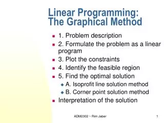
Topic – 7 Linear Programming: Simplex Method and Sensitivity Analysis. LP: Simplex Method and Interpretations. Some Important Questions about LP Model and Its Solutions: What is the impact if additional resources available? What if model parameters (cost/profit) change to LP solutions?

E N D
Topic – 7Linear Programming:Simplex Method and Sensitivity Analysis
LP: Simplex Method and Interpretations Some Important Questions about LP Model and Its Solutions: • What is the impact if additional resources available? • What if model parameters (cost/profit) change to LP solutions? • How to interpret LP solutions in managerial sense? Standardization of LP through Slack/Surplus/Artificial variables: • 1. Slack variables in "Resources" type constraints (≤): • How many resource i left in the solution? [Si ≥ 0] • (e.g. X1 + 2X2 ≤ 40 → X1 + 2X2 + S1 = 40) • If Si=0, "resource" i fully utilized (critical), and • If Si>0, some resource i are slack, available for other usage. • 2. Surplus variables in "Demand" type constraints (>): How much exceeds in "demand" i from Min-Requirement [Si ≥ 0] (e.g. X1 + 2X2 ≥ 40, → X1 + 2X2 - S2 = 40) If Si=0, demand i just meet minimum requirement, and If Si>0, demand i has exceeded the minimum requirement. • 3. Artificial variables in all ("≥" and "=") constraints: [ai≥ 0] To guarantee all variables ≥ 0 in solution searching process. (e.g. X1 + 2X2 ≥ 40, → X1 + 2X2 - S2 + a2 = 40, or (e.g. X1 + 2X2 = 40, → X1 + 2X2 + a2 = 40) ai itself no meaning, and must be out in final solution.
Simplex Solution Method Simplex is an iterative search algorithm for large LP problems, starting from the initial ("origin", all X = 0) and moving toward adjacent "corner" points at the direction in which improvement on objective function value is maximized. Key Property underlying Simplex: If one "corner" point solution is better than all adjacent "corner" point solutions, it is "optimal". Basic steps of Simplex Method: Iteration Process: (Tabular Form) • Initial Point: all X = 0 (non-basic), all Si = bi (basic) • One Xi (with max-contribution) enter - one Si leave out. • Repeat until the "optimal" is reached ("stop" rule). Special Cases in LP: • Degeneracy /Unbounded Solution /Unconstrained Variables • No Feasible Solution /Multi-Optimal /Redundant Constraints All these cases will be "automatically" detected in Simplex method.
LP Solution: Managerial Interpretations • How to interpret LP solutions in managerial sense? Shadow (Dual) Price: the marginal contribution (opportunity cost) of an additional unit of resource i to the objective function value under the given Upper and Lower limits of resource. • Is it worth to obtain additional resources from outside? • For the resource that has a slack > 0, its shadow price = 0. • For the resource that has a slack = 0, its shadow price > 0. In managerial sense, when the shadow price of resource i is greater than the cost to obtain, it is worth to obtain. • Shift slack resources (their shadow price = 0) to other activities. • Trade-off for re-allocation of resources among activities. • Exchange resources with smaller shadow prices for those with larger shadow prices. Graphical Interpretation: the resource constraints with a positive shadow price are Active (critical) constraints (the optimal solution pass through), while those with a zero shadow price are inactive constraints.
LP Solution: Sensitivity Analysis Sensitivity Analysis: concerns the impacts on optimal solution X* = {x*j, j=1,..n) if one or more given model parameters are changed due to market/supply/capacity/technology/.. changes. Objective Function Coefficients - Cj (j=1,...n) may be changed: • Graphically, Changes in Cj - will change the slope of objective function - which may or may not affect the optimal solution. • Managerial question: beyond what range of change (cost/profit) • (Lj ≤ Cj ≤ Uj) - X* (not Z) will be changed? • A larger range indicates insensitive of Z to changes in Cj. Reduced Cost (for variables with xj = 0 in the final solution): The amount of "cost" (In a MIN problem) to be reduced in order to make this variable back to solution with a positive value. (Or the amount of "profit" to be increased in a MAX problem). This information is also shown in the "Upper Limit" (Allowable Increase - Uj) or "Lower Limit" (Allowable Decrease - Lj) column in the solution printout.
Allowable Changing Range of Coefficients Resource Coefficients (RHS) - bi (i=1,...m) may be changed: • Graphically, changes in bi - will parallel shift the constraint line - which may or may not change the optimal solution: • change X* and Z if the constraint is active (Si = 0). • no change in X* and Z if the constraint is inactive (Si > 0). • Managerial question: beyond what range (BLi ≤ bi ≤ BUi) so X* will be changed? (considering possible "loosening"/increase or "tightening"/decrease in resource bi) Resource consumption coefficients - aij may be changed: • Graphically, changes in aij - will change the slope of constraint line (or parallel shift the constraint line up or down). The change will affect the optimal solution if the related constraint is an active constraint (Si = 0). • Managerial question: beyond what range (ALij≤ aij≤ BUij) so X* will be changed? (e.g., technological improvement or labor productivity increase) • All of the Upper and Lower limits for Cj, bi, and aij will be given in the Simplex solution.
When Adding or Deleting A Constraint: Will X* change? • Adding a new constraint - have two possibilities: • A redundant (inactive) one, no impact on X*, should remove it out. (Graphically, the new constraint line passing through outside of current feasible solution area.) • Reducing feasible solution area, may change X*, or not. • Otherwise, the feasible solution area is reduced, but the X* remains unchanged. • If new constraint line cuts out the optimal solution point from the original feasible solution area, the new X* needs to be calculated. (check by putting X* into new constraint) • Deleting an "old" constraint - also have two possibilities: If its slack Si = 0, active one, need to resolve problem. If its slack Si > 0, inactive one, no impact on X*.
LP: Dual Formation Duality: Prime vs. Dual: Counter-Expression of original LP • Duality: Symmetric and Reflexive relationship (a reflection of an object in the "Mirror"). • Max-Profit: by select Xi under resource constraints (bi), • Min-(opportunity) Cost - by select Yi under its contribution (cj). • Key Properties between Prime and its Dual: (Dual Theorem) • Same prime problem may have multiple dual formations. • Same problem, different Expression (Max ↔ Min). • Same optimal solution and objective function value. • The shadow prices of the prime is the decision variable value of the dual, and vice verse. (Principle of Complementary Slackness) • Formulation of the Dual from the Prime: • Standardize constraint set: • Max problem - all to (≤) type /Min problem, all to (≥). • Replace equality constraint with two inequality ones. • Transforming standardized Prime to Dual following rules. • No. of Variables in Dual = No. of Constraints in Prime • No. of Constraints in Dual = No. of Variables in Prime • Cj in Prime → bi in Dual / bi in Prime → Cj in Dual • aij in Prime → aji in Dual
Changes in the Technological Coefficient for the High Note Sound Company
Write the dual of the following problem: Min. z = 5x1 + 2x1 – 3x3 Subject to; 2x1 – x2 + 3x2≥ 60 x1 + 5x2 – 2x3 ≤ 50 2x1 + x3 = 15 Standardize the problem as a minimization and then write its dual.
Standardize: Max z = -5x1 - 2x1 + 3x3 Subject to: -2x1 + x2 - 3x2≤ -60 x1 + 5x2 - 2x3 ≤ 50 2x2 + x3 ≤ 15 -2x2 - x3 ≤ -15 Dual Min z= -60u1 + 50u2 + 15u3 – 15 u4 Subject to: -2u1 + u2≥ -5 u1 + 5u2 + 2u3 – 2u4≥ -2 -3u1 -2u2 + u3 –u4≥ 3
Or: Min z =-5x1 + 2x1 - 3x3 Subject to: 2x1- x2 + 3x2≥ -60 -x1 - 5x2 - 2x3 ≥ 50 2x2 + x3 ≥ 15 -2x2 - x3 ≥ -15 Dual Max z= 60u1 - 50u2 + 15u3 - 15 u4 Subject to: 2u1 - 1u2 + 0 u3 + 0u4 ≤ 5 -u1 - 5u2 + 2u3 – 2u4≤ 2 3u1 + 2u2 + u3 – u4≤ -3 Or: -3u1 -2u2 –u3 +u4≥ 3
Dual Formation: Economic Interpretations Why develop the Dual for the Prime Problem? a) Exhibit important economic/managerial interpretation: • Managerial information can be obtained directly from dual variables as from Shadow Price of resources in the Prime. • Dual model solution provides "opportunity cost" (Fair Price) for the constraints in the Prime. This information may offer many managerial insights for the original problem. • b) Provide basis for more efficient solution process. • The computational time of a LP problem is positively related to the number of constraints in the model. • For a LP problem with more constraints than variables, its dual problem has less constraints and more variables. In such a case, it is computational efficient to solve the dual problem than to solve the prime problem, especially for large sized problems. Duality has been widely used in many advanced MS models.
LP: Real World Applications • LP - is a very powerful, advanced, and complex MS technique used in all different fields and disciplines. • LP and its Simplex solution method provide basis for other advanced mathematical programming techniques (e.g., Integer Programming, Non-linear Programming). • There are many LP computer software packages available in the market with different functions and capabilities. • Major issues in real world LP applications: • Deviations from LP assumptions (e.g., Linearity/Nonnegative). • Difficult in collecting data and accuracy of data. • There may be many different formulations for the same problem. Specific formulation must be selected based on the purpose of the study and managerial considerations.