Download
1 / 40
410 likes | 524 Vues
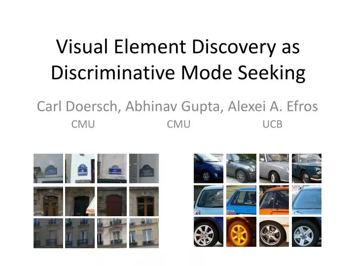
Visual Element Discovery as Discriminative Mode Seeking. CMU CMU UCB. Carl Doersch , Abhinav Gupta, Alexei A. Efros. The need for mid-level representations. 6 billion images. 70 billion images. 1 billion images served daily.

E N D
Visual Element Discovery as Discriminative Mode Seeking CMU CMU UCB Carl Doersch, Abhinav Gupta, Alexei A. Efros
The need for mid-level representations 6 billion images 70 billion images 1 billion images served daily 10 billion images 60 hours uploaded per minute : From Almost 90% of web traffic is visual!
Discriminative patches • Visual words are too simple • Objects are too difficult • Something in the middle? (Felzenswalb et al. 2008) (Singh et al. 2012)
Mid-level “Visual Elements” • Simple enough to be detected easily • Complex enough to be meaningful • “Meaningful” as measured by weak labels (Singh et al. 2012) (Doersch et al. 2012)
Mid-level “Visual Elements” • Doersch et al. 2012 • Singh et al. 2012 • Jain et al. 2013 • Endres et al. 2013 • Juneja et al. 2013 (Singh et al. 2012) (Doersch et al. 2012) • Li et al. 2013 • Sun et al. 2013 • Wang et al. 2013 • Fouhey et al. 2013 • Lee et al. 2013
Our goal • Provide a mathematical optimization for visual elements • Improve performance of mid-level representations.
What if the labels are weak? • E.g. image has horse/no-horse • (Or even weaker, like Paris/not-Paris) • Idea: Label these all as “horse” • Problem: 10,000 patches per image, most of which are unclassifiable.
The weaker the label, the bigger the problem. Task: Learn to classify Paris from Not-Paris Paris Also Paris
Other approaches • Latent SVM: • Assumes we have one instance per positive image • Multiple instance learning • Not clear how to define the bags
What if the labels are weak? • Negatives are negatives, positives might not be positive • Most of our data can be ignored • First: how to cluster without clustering everything (Singh et al. 2012) (Doersch et al. 2012)
Patch distances Input Nearest neighbor Min distance: 2.59e-4 Max distance: 1.22e-4
Paris Not Paris Negative Set
Paris Not Paris Negative Set
Paris Not Paris Density Ratios
Paris Not Paris Density Ratios
Positive Negative Adaptive Bandwidth Bandwidth
Discriminative Mode Seeking • Find local optima of an estimate of the density ratio • Allow an adaptive bandwidth • Be extremely fast • Minimize the number of passes through the data
Discriminative Mode Seeking • Mean shift: maximize (w.r.t. w) w Bandwidth Patch Feature Distance Centroid b
Discriminative Mode Seeking B(w) is the value of b satisfying:
Discriminative Mode Seeking • Distance metric: Normalized Correlation optimize s.t.
Positive Negative Discriminative Mode Seeking optimize s.t. w
Optimization • Initialization is straightforward • For each element, just keep around ~500 patches where wTx - b > 0 • Trivially parallelizable in MapReduce. • Optimization is piecewise quadratic s.t.
Evaluation via Purity-Coverage Plot • Analogous to Precision-Recall Plot
Low Purity Element 1 Element 2 Element 3 Element 4 Element 5
High purity, Low Coverage Element 1 Element 2 Element 3 Element 4 Element 5
Paris Not Paris Purity-Coverage Curve Purity x1e4 pixels Coverage
Paris Not Paris Purity-Coverage Curve Purity x1e4 pixels Coverage
Purity-Coverage Curve • Coverage for multiple elements is simply the union.
This work Purity-Coverage This work, no inter-element SVM Retrained 5x (Doersch et al. 2012) LDA Retrained 5x LDA Retrained Exemplar LDA (Hariharan et al. 2012) Top 25 Elements Top 200 Elements 1 0.98 0.96 0.94 0.92 Purity 0.9 0.88 0.86 0.84 0.82 0.8 0 0.1 0.2 0.3 0.4 0.5 0 0.2 0.4 0.6 0.8 Coverage (fraction of positive dataset) Coverage (fraction of positive dataset)
Results on Indoor 67 Scenes Kitchen Grocery Bowling Bakery Bathroom Elevator
Indoor67: Error Analysis Guess: staircase Guess: grocery store GT: corridor Ground Truth (GT): deli GT: laundromat GT: museum Guess: garage Guess: closet
Thank you! More results at http://graphics.cs.cmu.edu/projects/discriminativeModeSeeking/ Paris Elements • Indoor 67 Elements Indoor 67 Heatmaps• Source code (soon) Guess: staircase Guess: grocery store GT: corridor Ground Truth (GT): deli GT: laundromat GT: museum Guess: garage Guess: closet