Download
1 / 42
420 likes | 510 Vues
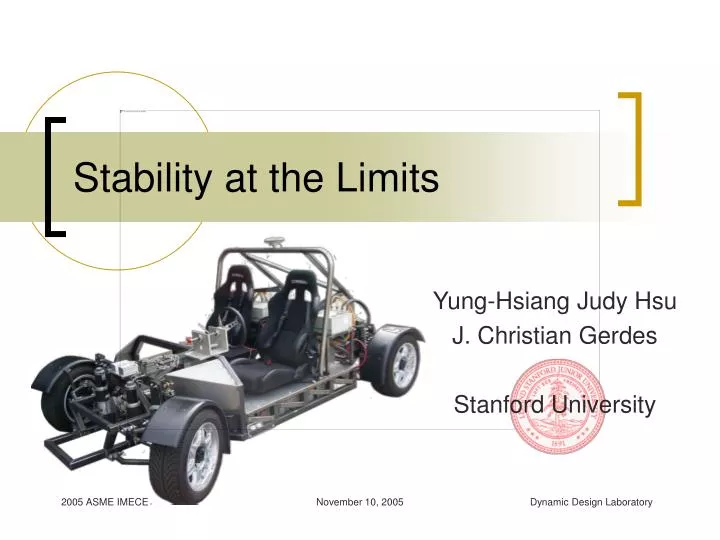
Stability at the Limits. Yung-Hsiang Judy Hsu J. Christian Gerdes Stanford University. did you know…. Every day in the US, 10 teenagers are killed in teen-driven vehicles in crashes 1 Loss of control accounts for 30% of these deaths

E N D
Stability at the Limits Yung-Hsiang Judy Hsu J. Christian Gerdes Stanford University November 10, 2005
did you know… • Every day in the US, 10 teenagers are killed in teen-driven vehicles in crashes1 • Loss of control accounts for 30% of these deaths • Inexperienced drivers make more driving errors, exceed speed limits & run off roads at higher rates • In 2002, motor vehicle traffic crashes were the leading cause of death for ages 3-33.2 To understand how loss of control occurs, need to know what determines vehicle motion 1 National Highway Traffic Safety Administration. Traffic safety facts (2002) 2 USA Today. Study of deadly crashes involving 16-19 year old drivers (2003) 2
motion of a vehicle SIDE VIEW • Motion of a vehicle is governed by tire forces • Tire forces result from deformation in contact patch • Lateral tire force is a function of tire slip Contact Patch Ground BOTTOM VIEW a Fy 3
tire curve maximum tire grip Linear Saturation Loss of control 4
vehicle response • Normally, we operate in linear region • Predictable vehicle response • But during slick road conditions, emergency maneuvers, or aggressive/performance driving • Enter nonlinear tire region • Response unanticipated by driver 5
loss of control Imagine making an aggressive turn • If front tires lose grip first, plow out of turn (limit understeer) • may go into oscillatory response • driver loses ability to influence vehicle motion • If rear tires saturate, rear end kicks out (limit oversteer) • may go into a unstable spin • driver loses control • Both can result in loss of control 6
overall goals We’d like to design a control system to • Stabilize vehicle in nonlinear handling region • Make vehicle response consistent and predictable for drivers • Communicate to driver when limits of handling are approaching 7
Outline • Identify tire operating region • Vehicle/Tire models • Tire parameter estimation • Produce stable, predictable response • Feedback linearizing controller • Driver input saturation • Simulation results 8
vehicle model Bicycle model • 2 states: β and r • Nonlinear tire model (Dugoff) • Steer-by-wire Assume • Small angles • Ux constant 9
equations of motion Sum forces and moments: Dugoff tire model: -C 10
tire estimation algorithm • Find f: use GPS/INS • Find Fyf: SBW motor give steering torque • Estimate C f and • LS fit to linear tire model • NLS fit to Dugoff model • Compare residual of fits to tell us if we’re in the nonlinear region estimate 11
parameter estimates • Begin estimating after entering NL region • C f estimate is steady 15
controller design • Desired vehicle response • Track response of bicycle model with linear tires • Be consistent with what driver expects • When tires saturate, compensate for decreasing forces with steer-by-wire input • One input f; two states ,r • Could compromise between the two • Or, track one state exactly 16
feedback linearization (FBL) • Nonlinear control technique Applicable to systems that look like: • Use input to cancel system nonlinearities. In our case, • Apply linear control theory to track desired trajectory: 17
FBL in action • Ramp steer from 0 to 4o at 20 m/s (45 mph) in 1 s • Controller results in exact tracking of linear tire model yaw rate trajectory 18
FBL in action • Ramp steer from 0 to 6o at 20 m/s (45 mph) in 1 s • FBL works well up to physical capabilities of tires 19
driver input saturation • Road naturally saturates driver’s steering capability often unexpectedly • Here, we safely limit steering capability in a predictable, safe manner • Why do we need it? • Prevents vehicle from needing more side force than is available • Keeps vehicle in linearizable handling region • Saturation algorithm • If < th, driver commands are OK • If ¸th, gradually saturate driver’s steering capability 20
overall control system • Ramp steer from 0 to 6° at 20 m/s (45 mph) in 1 s • Tracks linear model yaw rate, then saturates input • Reduced sideslip 21
design considerations • Relative importance of vs. r • Which produces a more predictable response? • Could add additional input to track and r • differential drive • rear steering 22
conclusions • Overall approach • Sense tire saturation and actively compensate for them with SBW inputs • Algorithm can characterize tires (C, ) using GPS-based f and estimates of Fyf, • Make vehicle response more predictable • Up to capabilities of tires, controller tracks linear yaw rate trajectory • Reduces sideslip • Current work • Estimate C, on board in real-time • Implement overall controller on research vehicle 23
controller validation • Simulate control system on more complete vehicle model 25
validation results II • input: ramp steer from 0 to 5° at 45 mph in 0.5 s 26
4 cases Case 1: Both tires are linear (f¸ 1 and r¸ 1) Case 2: Both tires saturating (f < 1 and r < 1) 27
4 cases Case 3: front is nonlinear, rear is linear (f¸ 1 and r < 1) Case 4: front is linear, rear is nonlinear (f¸ 1 and r < 1) 28
new inputs • Define new inputs v1 and v2 to represent system as 29
More general form of FBL SISO algorithm: 30
Front steering only approach • Model Fyf as: • Substitute into system equations: 32
Tracking yaw rate • Choose new input cr = 200 c = 50 33
Estimating Cf • Find f:Use GPS/INS to measure r and f and estimate • Find Fyf: Estimate tm from steering geometry, model tp as and use disturbance torque estimate from SBW system to find Fyf • Estimate : • Using least squares 34
Experimental Tire Curve • P1: Ramp steer from 0 to 9° in 24 s at V = 31 mph shad_2004-12-11_l.mat 35
questions? 36
overview • Motivation • Background • Controller design • Feedback linearization • Driver input saturation • Validation on complex model • Conclusions 37
steer-by-wire Removes mechanical linkage between steering wheel and road wheels • electronically actuate steering system separately from driver’s commands • decouple underlying dynamics from driver force feedback Conventional steering Steer-by-wire 38
comparing vehicle responses • Ramp steer to from 0 to 4o at 45 mph in 0.5 s 41
tire estimation algorithm • Find f: GPS/INS measures , r, V • Find Fyf: SBW motor give steering torque • Estimate C f and from (Fyf, f) data • LS fit to line • NLS fit to Dugoff Compare fit errors to tell us if in nonlinear region 42