Download
1 / 96
1.03k likes | 1.61k Vues
FPGA Routing. Dr. Philip Brisk Department of Computer Science and Engineering University of California, Riverside CS 223. Routing Resource Graph (RRG). source. wire 3. wire 4. 2-LUT. out. out. wire 3. wire 4. in 2. in 1. wire 2. wire 1. in 2. in 1. wire 1. wire 2. sink.

E N D
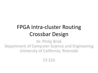
FPGA Routing Dr. Philip Brisk Department of Computer Science and Engineering University of California, Riverside CS 223
Routing Resource Graph (RRG) source wire3 wire4 2-LUT out out wire3 wire4 in2 in1 wire2 wire1 in2 in1 wire1 wire2 sink www.eecg.toronto.edu/~aling/ece1718/project/fang/route_rr_graph.png
FPGA Routing • Disjoint-path problem (on the RRG); NP-complete • Input: • Graph G(V, E) • Set of sources S = {s1, s2, …, sm} • Set of sets of sinks T = {T1, T2, …, Tn}, Ti= {ti1, ti2, …, tik} • Solution • Finds paths from each source si to all sinks in Ti • Paths emanating from different sinks must be disjoint (cannot shared any vertices or edges) • Objective(s) • Minimize delay, wirelength, etc.
Disjoint and Non-disjoint Paths s1 t21 s2 t11
Disjoint and Non-disjoint Paths Two nets are routed on the same FPGA segment (remember, RRG vertices represent wires and CLB I/Os) s1 t21 s2 t11 This route is illegal!
Disjoint and Non-disjoint Paths s1 t21 s2 t11 This route is legal!
LUT Input Equivalence (1/3) 2-LUT 2-LUT s1 s1 in1 in1 s2 s2 in2 in2 LUT inputs are interchangeable
LUT Input Equivalence (2/3) 2-LUT 2-LUT s1 s1 in1 in1 s2 s2 in2 in2 s1 s1 t11 = in1 t21 = in1 s2 s2 t21 = in2 t11 = in2 Overly restrictive disjoint-path problem formulation
LUT Input Equivalence (3/3) 2-LUT 2-LUT s1 s1 in1 in1 s2 s2 in2 in2 s1 t s2 Represent all inputs of a LUT as one RRG sink, t
PathFinder: A Negotiation-Based Performance-Driven Router for FPGAs Larry McMurchie and Carl Ebeling International Symposium on FPGAs, 1995
Architecture and CAD for Deep Submicron FPGAs(Section 2.2.3, pp. 25-30) Vaughn Betz, Jonathan Rose, Sandy Marquardt Springer, 1999
Basic Plan • Route nets one-by-one • Each net is routed by a priority-driven breadth-first search • Multiple nets may use the same nodes and edges • Node/edge costs depend on current usage and past usage history • Repeat for a fixed number of iterations (say 200) • Success: A disjoint routing solution for for all nets • Failure: No disjoint solution found after a fixed number of iterations
Routability Cost Function (per Node) • C(n) = p(n) × (b(n) + h(n)) • b(n): base cost of routing through node n • Typically the intrinsic delay of the circuit element corresponding to the node • h(n): history cost of routing through node n, based on previous router iterations • p(n): depends on the number of signals presently routed through node n in the current iteration
First-Order Congestion A 2 2 s1 t1 1 3 1 3 B 1 1 s2 t2 1 4 4 1 s3 t3 3 C 3
First-Order Congestion A 2 2 s1 t1 • All paths route through B • Increase the penalty cost of B per iteration due to sharing • In a future iteration, it will be cheaper to route signal 1 through A, rather than B • In a future iteration, it will be cheaper to route signal 2 through C, rather than B • Requires gradual increase in cost of sharing nodes 1 3 1 3 B 1 1 s2 t2 1 4 4 1 s3 t3 3 C 3
Second-order Congestion A 2 2 s1 Routing Order: 1, 2, 3 t1 1 1 B 2 2 s2 t2 1 1 s3 t3 1 C 1
Second-order Congestion A 2 2 s1 Routing Order: 1, 2, 3 t1 1 1 B 2 2 s2 t2 1 1 s3 t3 1 C 1
Second-order Congestion A 2 2 s1 Routing Order: 1, 2, 3 t1 1 1 B 2 2 s2 t2 1 1 s3 t3 1 C 1
Second-order Congestion A 2 2 s1 Routing Order: 1, 2, 3 t1 • Two paths route through C • Increasing the history cost through C will push signal 2 onto an alternative path through B 1 1 B 2 2 s2 t2 1 1 s3 t3 1 C 1
Second-order Congestion A 2 2 s1 Routing Order: 1, 2, 3 t1 • Two paths route through C • Increasing the history cost through C will push signal 2 onto an alternative path through B 1 1 B 2 2 s2 t2 3 3 s3 t3 3 C 3
Second-order Congestion A 2 2 s1 Routing Order: 1, 2, 3 t1 • Two paths route through B • Increasing the history cost through B will push signal 1 onto an alternative path through A • Increasing the history cost through B will push signal 2 back onto the path through C 1 1 B 2 2 s2 t2 3 3 s3 t3 3 C 3
Second-order Congestion A 2 2 s1 Routing Order: 1, 2, 3 t1 • Two paths route through B • Increasing the history cost through B will push signal 1 onto an alternative path through A • Increasing the history cost through B will push signal 2 back onto the path through C 3 3 B 4 4 s2 t2 3 3 s3 t3 3 C 3
Second-order Congestion A 2 2 s1 Routing Order: 1, 2, 3 t1 • Two paths route through C • Increasing the history cost through C will push signal 2 back through B 3 3 B 4 4 s2 t2 3 3 s3 t3 3 C 3
Second-order Congestion A 2 2 s1 Routing Order: 1, 2, 3 t1 • Two paths route through C • Increasing the history cost through C will push signal 2 back through B 3 3 B 4 4 s2 t2 5 5 s3 t3 5 C 5
Pseudocode • Priority driven BFS • Computed from the source to every sink of net(i) • Connect the newly found path to the current sink to the partly-computed routing tree RT(i) for net I
Timing-Routability Cost Function Delay of critical path • Represents the estimated criticality of the path from source I to sink j on net(i) • net(i) may fan out to multiple sinks with varying criticality, depending on placement
Negotiated A* Routing for FPGAs Russell Tessier Fifth Canadian Workshop on Field Programmable Devices, 1998
A* Cost Function • Cost at a node ni fi = gi + di gi= fi-1+ ci Estimated cost of routing from ni to the sink Cost of routing from the source to ni Cost of the next candidate node Total cost of previous path
A* vs. BFS A*:fi= gi + di = (fi-1 + ci) + di BFS: fi= gi Hybrid:fi = (1 - α)gi+ αdi = (1 - α)(fi-1 + ci)+ αdi
Good Ideas, But… • Algorithm and implementation assumed disjoint switch block • i.e., disjoint global routing domains • Key issue: • Which routing domains (reachable from the source) are explored in what order?
A Fast Routability-driven Router for FPGAs Jordan S. Swartz, Vaughn Betz, Jonathan Rose International Symposium on FPGAs, 1998
Architecture and CAD for Deep Submicron FPGAs(Section 4.3, pp. 76-80) Vaughn Betz, Jonathan Rose, Sandy Marquardt Springer, 1999
Speed Enhancements • Directed depth-first search • Similar to A*, but arguably more aggressive • Key Issues: • Cost function • Sink (target) ordering for multi-terminal nets • Route classification • Low-stress • Difficult • Impossible
Cost Function Cost(n) = C(n) + Costprev + α(ΔD) • Costprev: cost of track segments used to reach the current segment • C(n): (base) cost of using the track segment • Increases more rapidly than the original PathFinder algorithm • (ΔD): estimated cost of routing from the current track segment to the destination • Based on Manhattan (XY) distance) • α: Direction factor • BFS: α = 0 • Directed search: α > 0
Updated Node (Base) Cost Function • C(n) = p(n) × (b(n) + h(n)) • b(n): base cost • h(n): history cost • p(n): usage cost • C(n) = p(n) × b(n) × h(n) + Bendcost(n, m) • Multiplying b(n) and h(n) eliminates normalization • Penalize global routes that take a lot of turns • These routes are less likely to use long wires
Penalty Cost Function • Not specified in the original PathFinder paper p(n) = 1 + max(0, [occupancy(n) – capacity(n)] × pfac) • occupancy(n): number of nets using resource n • capacity(n): maximum number of nets that can use resource n (typically 1) • pfac: 0.5 for the first iteration; increase by 1.5x to 2x each subsequent iteration
History Cost Function • Not specified in the original PathFinder paper • occupancy(n): number of nets using resource n • capacity(n): maximum number of nets that can use resource n (typically 1) • hfac: constant; any value between 0.2 and 1 works well
Target Selection • Closest Sink First • Uses fewer track segments • Furthest Sink First • Uses more track segments
Net Order • Route nets in order of decreasing fan-out • High fanout nets tend to span the whole FPGA • Easier to route when there is less congestion do to other nets routed earlier • Low fanout nets tend to be more localized • Relatively easy to route, even in the presence of some congestion
Binning • Only the portions of the net close to the target sink should be expanded • E.g., only expand within Bin 4 in this example • Shown to be effective for sinks with more than 50 targets
Bounding Box • Define a bounding box around source and sinks • Restrict the route for each net to no more than 3 channels outside of the bounding box
Difficulty Prediction • Since you can’t know Wmin first without routing, use an estimate based on a wirelength prediction model
Difficulty Prediction • Westimate took less than 1 second to compute • Some prediction mistakes will happen • Prediction accuracy was 84%