Download
1 / 10
100 likes | 263 Vues
EE359 – Lecture 6 Outline. Announcements: No lecture Mon, lectures 10/19 6pm, 10/21 9:30am HW this week deadline extended to Friday 5pm Next HW posted today, due Friday 10/21@5pm Review of Last Lecture Signal Envelope Distributions Average Fade Duration Markov Models

E N D
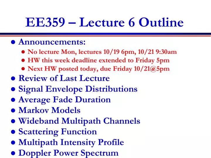
EE359 – Lecture 6 Outline • Announcements: • No lecture Mon, lectures 10/19 6pm, 10/21 9:30am • HW this week deadline extended to Friday 5pm • Next HW posted today, due Friday 10/21@5pm • Review of Last Lecture • Signal Envelope Distributions • Average Fade Duration • Markov Models • Wideband Multipath Channels • Scattering Function • Multipath Intensity Profile • Doppler Power Spectrum
Review of Last Lecture • For fn~U[0,2p], rI(t),rQ(t) zero mean, WSS, with • Uniform AoAs in Narrowband Model • In-phase/quad comps have zero cross correlation and • PSD is maximum at the maximum Doppler frequency • PSD used to generate simulation values Decorrelates over roughly half a wavelength
Signal Envelope Distribution • CLT approx. leads to Rayleigh distribution (power is exponential) • When LOS component present, Ricean distribution is used • Measurements support Nakagami distribution in some environments • Similar to Ricean, but models “worse than Rayleigh” • Lends itself better to closed form BER expressions
Level crossing rate and Average Fade Duration • LCR: rate at which the signal crosses a fade value • AFD: How long a signal stays below target R/SNR • Derived from LCR • For Rayleigh fading • Depends on ratio of target to average level (r) • Inversely proportional to Doppler frequency t1 t2 t3 R
Markov Models for Fading R2 A2 R1 A1 R0 A0 • Model for fading dynamics • Simplifies performance analysis • Divides range of fading power into discrete regions Rj={g: Aj g < Aj+1} • Aj s and # of regions are functions of model • Transition probabilities (Lj is LCR at Aj):
t t Wideband Channels • Individual multipath components resolvable • True when time difference between components exceeds signal bandwidth Narrowband Wideband
Scattering Function • Fourier transform of c(t,t) relative to t • Typically characterize its statistics, since c(t,t) is different in different environments • Underlying process WSS and Gaussian, so only characterize mean (0) and correlation • Autocorrelation is Ac(t1,t2,Dt)=Ac(t,Dt) • Statistical scattering function: r s(t,r)=FDt[Ac(t,Dt)] t
Multipath Intensity Profile Ac(t) • Defined as Ac(t,Dt=0)= Ac(t) • Determines average (TM ) and rms (st) delay spread • Approximate max delay of significant m.p. • Coherence bandwidth Bc=1/TM • Maximum frequency over which Ac(Df)=F[Ac(t)]>0 • Ac(Df)=0 implies signals separated in frequency by Df will be uncorrelated after passing through channel TM t Ac(f) f t Bc 0
Doppler Power Spectrum Sc(r) • Sc(r)=F[Ac(t=0,Dt)]= F[Ac(Dt)] • Doppler spread Bd is maximum doppler for which Sc (r)=>0. • Coherence time Tc=1/Bd • Maximum time over which Ac(Dt)>0 • Ac(Dt)=0 implies signals separated in time by Dt will be uncorrelated after passing through channel r Bd
Main Points • Fading distribution depends on environment • Rayleigh, Ricean, and Nakagami all common • Average fade duration determines how long a user is in continuous outage (e.g. for coding design) • Markov model approximates fading dynamics. • Scattering function characterizes rms delay and Doppler spread. Key parameters for system design. • Delay spread defines maximum delay of significant multipath components. Inverse is coherence BW • Doppler spread defines maximum nonzero doppler, its inverse is coherence time