Eddy distribution around the Zapiola Drift area in the Southwestern Atlantic

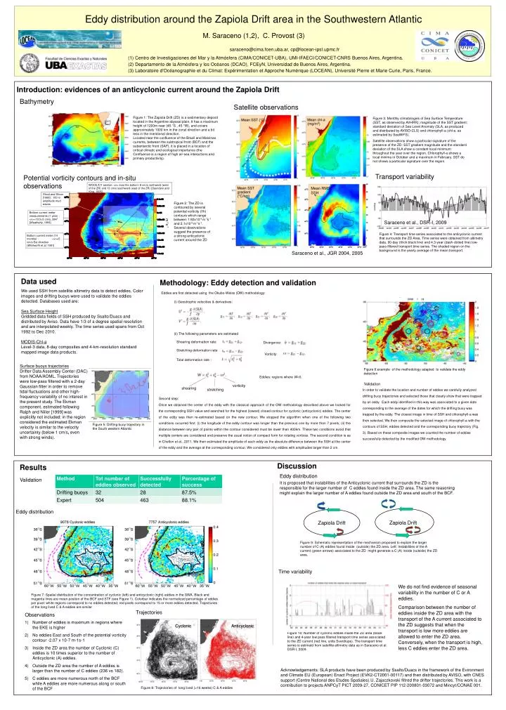
1. vorticity shearing stretching Eddy distribution around the Zapiola Drift area in the Southwestern Atlantic M. Saraceno (1,2), C. Provost (3) saraceno@cima.fcen.uba.ar, cp@locean-ipsl.upmc.fr (1) Centro de Investigaciones del Mar y la Atmósfera (CIMA/CONICET-UBA), UMI-IFAECI/CONICET-CNRS Buenos Aires, Argentina. (2) Departamento de la Atmósfera y los Océanos (DCAO), FCEyN, Universidad de Buenos Aires, Argentina. (3) Laboratoire d'Océanographie et du Climat: Expérimentation et Approche Numérique (LOCEAN), Université Pierre et Marie Curie, Paris, France. Introduction: evidences of an anticyclonic current around the Zapiola Drift Bathymetry Satellite observations Figure 1: The Zapiola Drift (ZD) is a sedimentary deposit located in the Argentine abyssal plain. It has a maximum height of 1200m near (45 °S , 45 °W), and covers approximately 1000 km in the zonal direction and a bit less in the meridional direction. Located near the confluence of the Brazil and Malvinas currents, between the subtropical front (BCF) and the subantarctic front (SAF), it is placed in a location of critical climatic and ecological importance (the Confluence is a region of high air-sea interactions and primary productivity). Figure 3: Monthly climatologies of Sea Surface Temperature (SST, as observed by AVHRR); magnitude of the SST gradient; standard deviation of Sea Level Anomaly (SLA, as produced and distributed by AVISO-CLS) and chlorophyll-a (chl-a, as estimated by SeaWiFS). Satellite observations show a particular signature of the presence of the ZD: SST gradient magnitude and the standard deviation of the SLA show a constant local minimum throughout the year over the region. Chlorophyll-a shows a local minima in October and a maximum in February. SST do not shows a particular signature over the region. Transport variability Potential vorticity contours and in-situ observations WOCE A11 section: <v> near the bottom: 8 cm/s northward (west of the ZR) and 13 cm/s southward (east of the ZR) [Saunders and King, 1995] Mean RMS SSH Flood and Shoor [1988] : 100 m amplitude mud waves Figure 2: The ZD is contoured by several potential vorticity (f/h) contours which range between 1.92x10-8 m-1s-1 and 2.1x10-8 m-1s-1. Several observations suggest the presence of a strong anticyclonic current around the ZD Bottom current meter measurements (1 year) : <v>=10.55 cm/s, 284° [Weatherly, 1993] Saraceno et al., DSR-I, 2009 m-1s-1 Figure 4: Transport time series associated to the anticyclonic current that surrounds the ZD Area. Time series were obtained from altimetry data. 90-day (thick black line) and 4.3-year (dash-dotted line) low-pass-filtered transport time series. The shaded region on the background is the yearly average of the mean transport. Bottom current meter (14 months) : <v>=5 cm/s Est direction [Whitworth et al, 1991] Saraceno et al., JGR 2004, 2005 Data used Methodology: Eddy detection and validation We used SSH from satellite altimetry data to detect eddies. Color images and drifting buoys were used to validate the eddies detected. Databases used are: Sea Surface Height Gridded data fields of SSH produced by Ssalto/Duacs and distributed by Aviso. Data have 1/3 of a degree spatial resolution and are interpolated weekly. The time series used spans from Oct 1992 to Dec 2010. MODIS-Chl-a Level-3 data, 8-day composites and 4-km-resolution standard mapped image data products. Eddies are first detected using the Okubo-Weiss (OW) methodology: (i) Geostrophic velocities & derivatives: (ii) The following parameters are estimated Shearing deformation rate: Divergence: Stretching deformation rate Vorticity: Total deformation rate : Surface buoys trajectories Drifter Data Assembly Center (DAC) from NOAA/AOML. Trajectories were low-pass filtered with a 2-day Gaussian filter in order to remove tidal fluctuations and other high-frequency variability of no interest in the present study. The Ekman component, estimated following Ralph and Niiler [1999] was explicitly not included: in the region considered the estimated Ekman velocity is similar to the velocity uncertainty (below 1 cm/s, even with strong winds). Figure 6:example of the methodology adapted to validate the eddy detection Eddies: regions where W<0. Validation In order to validate the location and number of eddies we carefully analyzed drifting buoy trajectories and selected those that clearly show that were trapped by an eddy. Each eddy identified in this way was associated to a given date corresponding to the average of the dates for which the drifting buoy was trapped by the eddy. The closest image in time of SSH and chlorophyll-a was then selected. We then composite the selected image of chlorophyll-a with the contours of SSH, eddies detected and the corresponding buoy trajectory (Fig. 3). Based on these composite images we counted the number of eddies successfully detected by the modified OW methodology. Second step: Once we obtained the center of the eddy with the classical approach of the OW methodology described above we looked for the corresponding SSH value and searched for the highest (lowest) closed contour for cyclonic (anticyclonic) eddies. The center of the eddy was then re-estimated based on the new contour. We stopped the algorithm when one of the following two conditions occurred first: (i) the longitude of the eddy contour was longer than the previous one by more than 7 pixels; (ii) the distance between any pair of points within the contour considered must be lower than 400km. These two conditions avoid that multiple centers are considered and preserve the usual notion of compact form for rotating vortices. The second condition is as in Chelton et al., 2011. We then estimated the amplitude of each eddy as the absolute difference between the SSH at the center of the eddy and the average at the corresponding contour. We considered only eddies with amplitudes larger than 2 cm. Figure 5: Drifting buoy trajectory in the South western Atlantic Discussion Results Eddy distribution Validation It is proposed that instabilities of the Anticyclonic current that surrounds the ZD is the responsible for the larger number of C eddies found inside the ZD area. The same reasoning might explain the larger number of A eddies found outside the ZD area and south of the BCF. Eddy distribution Zapiola Drift Zapiola Drift Figure 9: Schematic representation of the mechanism proposed to explain the larger number of C (A) eddies found inside (outside) the ZD area. Left: Instabilities of the A current (green arrows) associated to the ZD might generate a C (A) inside (outside) the ZD area. Time variability We do not find evidence of seasonal variability in the number of C or A eddies. Comparison between the number of eddies inside the ZD area with the transport of the A current associated to the ZD suggests that when the transport is low more eddies are allowed to enter the ZD area. Conversely, when the transport is high, less C eddies enter the ZD area. Figure 7: Spatial distribution of the concentration of cyclonic (left) and anticyclonic (right) eddies in the SWA. Black and magenta lines are mean postion of the BCF and STF (see Figure 1). Colorbar indicates the normalized percentage of eddies per pixel: white regions correspond to no eddies detected; red pixels correspond to 15 or more eddies detected. Trajectories of the long lived C & A eddies are similar Trajectories Observations Number of eddies is maximum in regions where the EKE is higher No eddies East and South of the potential vorticity contour -2.07 x 10-7 m-1s-1 Inside the ZD area the number of Cyclonic (C) eddies is 10 times superior to the number of Anticyclonic (A) eddies. Outside the ZD area the number of A eddies is larger than the number of C eddies (236 vs 182). C eddies are more numerous north of the BCF while A eddies are more numerous along or south of the BCF Cyclonic Anticyclonic Figure 10: Number of cyclonic eddies inside the ZD area (black line) and 4-year low pass filtered transport time series associated to the ZD current (red line, units Sverdrups). The transport time series is estimatd from satellite altimetry data as in Saraceno et al. DSR-I, 2009. Acknowledgements: SLA products have been produced by Ssalto/Duacs in the framework of the Evironment and Climate EU (European) Enact Project (EVK2-CT2001-00117) and then distributed by AVISO, with CNES support (Centre National des Etudes Spatiales).U. Zajaczkovski filtred the drifter trajectories. This work is a contribution to projects ANPCyT PICT 2009-27, CONICET PIP 112-200801-03072 and Mincyt/CONAE 001. Figure 8: Trajectories of long lived (>16 weeks) C & A eddies