Download
1 / 38
410 likes | 576 Vues
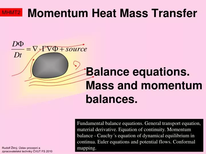
Momentum Heat Mass Transfer. MHMT2. Balance equations. Mass and momentum balances.

E N D
Momentum Heat Mass Transfer MHMT2 Balance equations. Mass and momentum balances. Fundamental balance equations. General transport equation, material derivative. Equation of continuity. Momentum balance - Cauchy´s equation of dynamical equilibrium in continua. Euler equations and potential flows. Conformal mapping. Rudolf Žitný, Ústav procesní a zpracovatelské techniky ČVUT FS 2010
Mass-Momentum-Energy MHMT2 Mechanics and thermodynamics are based upon the • Conservation laws • -conservation of mass • conservation of momentum M.du/dt=F (second Newton’s law) • conservation of energy dq=du+pdv (first law of thermodynamics) • Transfer phenomena summarize these conservation laws and applies them to a continuous system described by macroscopic variables distributed in space (x,y,z) and time (t) Description of kinematics and dynamics of discrete mass points is recasted to consistent tensor form of integral or partial differential equations for velocity, temperature, pressure and concentration fields.
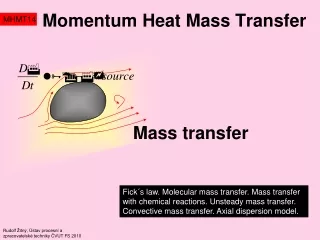
Transported property MHMT2 Transfer phenomena looks for analogies between transport of mass, momentum and energy. Transported properties are scalars (density, energy) or vectors (momentum). Fluxes are amount of passing through a unit surface at unit time (fluxes are tensors of one order higher than the corresponding property , therefore vectors or tensors). Convective fluxes ( transported by velocity of fluid) Diffusive fluxes ( transported by molecular diffusion) Driving forces = gradients of transported properties
Transported property MHMT2 This table presents nomenclature of transported properties for specific cases of mass, momentum, energy and component transport. Similarity of constitutive equations (Newton,Fourier,Fick) is basis for unified formulation of transport equations.
Mass conservation(fixed fluid element) MHMT2 Mass conservation principle can be expressed by balancing of a control volume (rate of mass accumulation inside the control volume is the sum of convective fluxes through the control volume surface). Analysis is simplified by the fact that the molecular fluxes are zero when considering homogeneous fluid. Control volumes can be fixed in space or moving.The simplest case, directly leading to the differential transport equations, is based upon identification of fluxes through sides of an infinitely small FLUID ELEMENTfixed in space.
Accumulation of mass Mass flowrate through sides W and E z y Top North East West South x z y x Bottom x Mass conservation(fixed fluid element) MHMT2 Using the control volume in form of a brick is straightforward but clumsy. However, tensor calculus is not necessary.
Mass conservation(fixed fluid element) MHMT2 Using index or symbolic notation makes equations more compact Continuity equation written in the index notation (Einstein summation is used) Continuity equation written in the symbolic form (Gibbs notation) Example: Continuity equation for an incompressible liquid is very simple
Time rate changes of MHMT2 Observer (an instrument measuring the property ) can be fixed in space and then the recorded rate od change is fixed observer measuring velocity of wind 10 km/h Rate of change of property (t,x,y,z) recorded by the observer moving at velocity running observer Total derivative Time changes of recorded by observer moving at velocity 20 km/h Material derivative is a special case of the total derivative, corresponding to the observer moving with the particle (with the same velocity as the fluid particle) observer in a balloon 0 km/h
Balancing in a fixed fluid element and material derivative MHMT2 intensity of inner sources or diffusional fluxes across the fluid element boundary [Accumulation in FE ] + [Outflow of from FE by convection] = This follows from the mass balance These terms are cancelled
ds V Integral balance of (fixed CV) MHMT2 Integral balance in a fixed control volume has the advantage that it is possible to exchange a time derivative and integration operator(V is independent of time) apply Gauss theorem (conversion of surface to volume integral)
Differential balance of MHMT2 Integral balance should be satisfied for arbitrary volume V Therefore integrand must be identically zero Remark: special case is the mass conservation for =1 and zero source term and using this the differential balance can be expressed in the alternative form
Momentum conservation MHMT2 Momentum balance = balance of forces is nothing else than the Newton’s law m.du/dt=F applied to continuous distribution of matter, forces and momentum. Newton’s law expressed in terms of differential equations is called CAUCHY’S equation valid for fluids and solids (exactly the same Cauchy’s equations hold in solid and fluid mechanics). Modigiani
external forces, like gravity source Momentum integral balance MHMT2 MOMENTUMintegral balances follow from the general integral balances for total stress viscous stress
Momentum conservation MHMT2 Differential equations of momentum conservation can be derived directly from the previous integral balance which must be satisfied for any control volume V, therefore also for any infinitely small volume surrounding the point (x,y,z) and [N/m3] This is the fundamental result, Cauchy’s equation (partial parabolic differential equations of the second order). You can skip the following shaded pages, showing that the same result can be obtained by the balance of forces.
Cauchy’s Equations MHMT2 Cauchy’s equation holds for solid and fluids (compressible and incompressible) formulation with primitive variables,u,v,w,p. Suitable for numerical solution of incompressible flows (Ma<0.3) Ma-Mach number (velocity related to speed of sound) Making use the previously derived relationship the Cauchy’s equation can be expressed in form conservative formulation using momentum as the unknown variable is suitable for compressible flows, shocks…. Passage through a shock wave is accompanied by jump of p,,u but (u) is continuous. These formulations are quite equivalent (mathematically) but not from the point of view of numerical solution – CFD.
Euler’s Equations inviscid flows MHMT2 Inviscid flow theory of ideal fluids is very highly mathematically developed and predicts successfully flows around bodies, airfoils, wave motion, Karman vortex street, jets. It fails in the prediction of drag forces.
Euler’s Equations and velocity potential MHMT2 Eulers’s equations are special case of Cauchy’s equations for inviscible fluids (therefore for zero viscous stresses) Vorticity vector describes rotation of velocity field and is defined as for example the z-coordinate of vorticity is Using vorticity the Euler equation can be written in the alternative form this formulation shows, that for zero vorticity the Euler’s equation reduces to Bernoulli’s equation: acceleration+kinetic energy=pressure drop+external forces Proof is based upon identity: see lecture 1.
Euler’s Equations and velocity potential MHMT2 Inviscid flows are frequently solved by assuming that velocity fields and volumetric forces f can be expressedas gradients of scalar functions (velocity potential) Vorticity vector of any potential velocity field is zero (potential flow is curl-free) because to understand why, remember that for the Levi Civita tensor holds imn= -inm Velocities defined as gradients of potential automatically satisfy Kelvins theorem stating that if the fluid is irrotational at any instant, it remains irrotational thereafter (holds only for inviscible fluids!). Because vorticity is zero the Euler equation is simplified … integrating along a streamline gives Bernoulli’s equation
Euler’s Equations and stream function MHMT2 In 2D flows it is convenient to introduce another scalar function, stream function Velocity derived from the scalar stream function automatically satisfies the continuity equation (divergence free or solenoidal flow) because Curves =const are streamlines, trajectories of flowing particles. For example solid boundaries are also streamlines. Difference is the fluid flowrate between two streamlines. Advantages of the stream function appear in the cases that the flow is rotational due to viscous effects (for example solid walls are generators of vorticity). In this case the dynamics of flow can be described by a pair of equations for vorticity and stream function In this way the unknown pressure is eliminated and instead of 3 equations for 3 unknowns ux uy p it is sufficient to solve 2 equations for and .
Problem of inviscid incompressible flows can be reduced to the solution of two Laplace equations for stream and potential functions, satisfying boundary conditions of impermeable walls ( ) and zero vorticity at inlet/outlet (). Euler’s Equations vorticity and stream function MHMT2 Let us summarize: For incompressible (divergence-free) flows the velocity potential distribution is described by the Laplace equation (ensures continuity equation) For irrotational (curl-free) flow the stream function should also satisfy the Laplace equation
U r Euler’s Equations flow around sphere MHMT2 Example: Velocity field of inviscid incompressible flow around a sphere of radius R is a good approximation of flows around gas bubbles, when velocity slips at the sphere surface. Velocity potential can be obtained as a solution of the Laplace equation written in the spherical coordinate system (r,,) Velocity potencial satisfying boundary condition at r and zero radial velocity at surface is The solution is found by factorisation to functions depending on r and on only and velocities (gradient of ) Velocity profile at surface (r=R) determines pressure profile (Bernoulli’s equation)
U r Euler’s Equations flow around cylinder MHMT2 Example: Potencial flow around cylinder can be solved by using velocity potencial function or by stream function. Both these functions have to satisfy Laplace equation written in the cylindrical coordinate system (the only difference is in boundary conditions). Stream function satisfying boundary condition at r (uniform velocity U) and constant at surface is see the result obtained by using complex functions giving radial and tangential velocities Compare with the previous result for sphere: the velocity decays with the second power of radius for cylinder, while with the third power at sphere (which could have been expected).
y x Euler’s Equations and complex functions MHMT2 Many interesting solutions of Euler’s equations can be obtained from the fact that the real and imaginary parts of ANY analytical function satisfy the Laplace equation (see next page). z=x+iy is a complex variable (i-imaginary unit) and w(z)=(x,y)+i(x,y) is also a complex variable (complex function), for example This is important statement: Quite arbitrary analytical function describes some flow-field. Real part of the complex variable w is velocity potential and the imaginary part Im(w) is stream function! Simple analytical functions describe for example sinks, sources, dipoles. In this way it is possible to solve problems with more complicated geometries, for example free surface flows, flow around airfoils, see applications of conformal mapping. Conformal mapping =const streamlines w(z) z(w) =const Equipotential lines
Euler’s Equations and complex functions MHMT2 Derivative dw/dz of a complex function w(z=x+iy)=+i with respect to z can be a complex analytical function as soon as both Re(w), Im(w) satisfy the Laplace equation Result should be independent of the dx, dy selection, therefore dy=0 dx=0 and this requirement is fulfilled only if both functions , satisfy Cauchy-Riemann conditions and therefore
Euler’s Equations and complex functions MHMT2 The real and the imaginary part of derivative dw/dz determine components of velocity field y x y x y x dipole x y source x y circulation x
=1 =-3 =0 =3 =0.5 =0.1 Euler’s Equations and complex functions MHMT2 Example: Let’s consider the transformation w(z)=az2 in more details Equipotential lines Stream lines The same graph can be obtained from inverse transformation z(w)
Euler’s Equations and complex functions MHMT2 • The following examples demonstrate the most important techniques used for construction of conformal mappings • Potential flow around circular cylinder with circulation (using directory of basic transformations, see previous slide – application of superposition principle: sum of analytical functions is also an analytical function) • Potential flow around an elliptical cylinder (making use conformal mapping of ellipse to circle, based upon Laurent series expansion – this is application of the substitution principle: analytical function of an analytical function is also an analytical function) • Cross flow around a plate (or how to transform an arbitrary polygonal region into upper half plane of complex potential – Schwarz Christoffel theorem) • Flows with free surface (contraction flow from an infinitely large reservoire through a slit)
Euler’s Equations cylinder with circulation MHMT2 Example: Potential flow around cylinder with circulation can be assumed as superposition of linear parallel flow w1(z)=Uz, dipole w2(z)=UR2/z and potential swirl w3(z)=/(2i) ln z (see the previous table). Substituting coordinates x,y by radius r and angle results into (x+iy=r ei) Comparing real and imaginary part potential and stream functions are identified velocity potential is the real part of the analytical function w(z) stream function is the imaginary part of the analytical function w without circulation, I have a problem in Matlab
Euler’s Equationselliptic cylinder MHMT2 Example: Potential flow around elliptic cylinder. Previous example solved the problem of potential flow around a cylinder with radius R, described by the conformal mapping The analytical function transforming outside of an elliptical cylinder to the plane of complex potential w= +i can be obtained in two steps: First step is a conformal mapping (z) transforming ellipse with principal axis a,b to a cylinder with radius a+b. The second step is substitution of the mapping (z) to the velocity potential There exist many techniques how to identify the conformal mapping (z) transforming a general closed region in the z=x+iy plane into a unit circle, for example numerically or in terms of Laurent series …this is the way how to solve the problems of flow around profiles, for example airfoils. It is just only necessary to find out a conformal mapping transforming the profile to a circle.
Euler’s Equationselliptic cylinder MHMT2 Im y -plane Z-plane x b Re a+b a For the conformal mapping of ellipse only three terms of Laurent’s series are sufficient with Inversion mapping (z) is the solution of quadratic equation Complex potential (potential and stream function) is therefore
Euler’s Equations conformal mapping MHMT2 Generally speaking it does not matter if we select analytical function w(z) mapping the spatial region (z=x+iy) to complex potential region w=+i, or vice versa. This is because inverse mapping is also conformal mapping.
Euler’s Equationscross flow around a plate MHMT2 Please notice the fact, that in this case the role of z and w is exchanged, complex variable w is spatial coordinates x,y, while z=+i is complex potential of velocity field. Solution for h=1 by MATLAB =1 fi=linspace(-10,10,1000); for psi=0.1:0.1:1 z=complex(fi,psi); w=(z.^2-1).^0.5; plot(w); hold on; end =0.1 See M.Sulista: Analyza v komplexnim oboru, MVST, XXIII, 1985, pp.100-101.
Euler’s Equations 3D stream function MHMT2 Disadvantage of the approach using stream function, complex variables and conformal mapping is its limitation to 2D flows. While in the 3D flow the irrotational velocity field can be described by only one scalar function , description of 3D solenoidal field (satisfying continuity equation) by stream function is not so simple. It is necessary to use a generalized stream function vector and to decompose velocities into curl free and solenoidal components (dual potential approach) Divergence free (solenoidal flow) Curl free (potential flow) Vorticity vector is expressed in terms of the stream function vector using identity The dual potential approach increases number of unknowns (3 stream functions and 2 vorticity transport equations are to be solved) and is not so frequently used.
Euler’s Equations MHMT2 Simple questions • Let the scalar function (t,x1,x2) satisfies Laplace equation. Does it mean that the gradient of this function represents velocity field satisfying both Euler equations in the directions x1,x2? The answer is positive. • Is it possible that a velocity field satisfying the Euler’s equations and the continuity equation is rotational (therefore cannot be expressed as a gradient of potential)? Answer is positive again.
EXAM MHMT2 Transport equations
What is important (at least for exam) MHMT2 You should know what is it material derivative Balancing of fluid particle Balancing of fixed fluid element Reynolds transport theorem
What is important (at least for exam) MHMT2 Continuity equation and Cauchy’s equations Euler’s equation Bernoulli’s equation
What is important (at least for exam) MHMT2 What is it vorticity, stream function and velocity potential Special case for 2D flows Complex potential, analytical functions and conformal mapping