Download
1 / 23
230 likes | 380 Vues
Computer Architecture Parallel Processors. Taxonomy. Flynn’s Taxonomy Classify by Instruction Stream and Data Stream SISD Single Instruction Single Data Conventional processor SIMD Single Instruction Multiple Data One instruction stream Multiple data items Several Examples Produced

E N D
Computer Architecture Parallel Processors
Taxonomy • Flynn’s Taxonomy • Classify by Instruction Stream and Data Stream • SISD Single Instruction Single Data • Conventional processor • SIMD Single Instruction Multiple Data • One instruction stream • Multiple data items • Several Examples Produced • MISD Multiple Instruction Single Data • Systolic Arrays (according to Hwang) • MIMD Multiple Instruction Multiple Data • Multiple Threads of execution • General Parallel Processors
SIMD - Single Instruction Multiple Data • Originally thought to be the ultimatemassively parallel machine! • Some machines built • Illiac IV • Thinking Machines CM2 • MasPar • Vector processors (special category!)
SIMD - Single Instruction Multiple Data • Each PE is asimple ALU(1 bit in CM-1,small processor in some) • Control Procissues sameinstruction toeach PE in eachcycle • Each PE has different data
SIMD • SIMD performance depends on • Mapping problem ð processor architecture • Image processing • Maps naturally to 2D processor array • Calculations on individual pixels trivial • Combining data is the problem! • Some matrix operations also
SIMD Note the B matrix is transposed! • Matrix multiplication • Each PE • * then • + • PEijð Cij
Parallel Processing • Communication patterns • If the system provides the “correct” data paths,then good performance is obtainedeven with slow PEs • Without effective communicationbandwidth,even fast PEs are starved of data! • In a multiple PE system, we have • Raw communication bandwidth • Equivalent processor ó memory bandwidth • Communications patterns • Imagine the Matrix Multiplication problem if the matrices are not already transposed! • Network topology
Systolic Arrays • Arrays of processors which pass data from one to the next at regular intervals • Similar to SIMD systems • But each processor may perform a different operation • Applications • Polynomial evaluation • Signal processing • Limited as general purpose processors • Communication pattern requiredneeds to match hardware links provided(a recurring problem!)
Systolic Array - iWarp • Linear array of processors • Communication links in forward and backward directions
Systolic Array - iWarp • Polynomial evaluation is simple • Use Horner’s rule • PEs - in pairs • multiply input by x, • passes result to right • add aj to result from left • passes result to right y = ((((anx + an-1)*x + an-2)*x + an-3)*x …… a1)*x + a0
Systolic Array - iWarp • Similarly FFT is efficient • DFT • n2 operations needed for n-element DFT • FFT • Divides this into 2 smaller transforms • algorithm with log2n phases of n operations • Total n log2n • Simple strategy with log2n PEs yj = S akwkj yj = S a2mw2mj + wj S a2m+1w2mj n/2 “even” terms n/2 “odd” terms
Systolic Arrays - General • Variations • Connection topology • 2D arrays, Hypercubes • Processor capabilities • Trivial - just an ALU • ALU with several registers • Simple CPU - registers, runs own program • Powerful CPU - local memory also • Reconfigurable • FPGAs, etc • Specialised applications only • Problem “shape” maps to interconnect pattern
Vector Processors - The Supercomputers • Optimised for vector & matrix operations “Conventional” scalar processor section not shown
Vector Processors - Vector operations • Example • Dot product or in terms of the elements • Fetch each element of each vector in turn • Stride • “Distance” between successive elements of a vector • 1 in dot-product case y = A l B y = Sak * bk
Vector Processors - Vector operations • Example • Matrix multiply or in terms of the elements C = A B cij = Saik * bkj
Vector Operations • Fetch data into vector register • Address Generation Unit manages stride Very high effectivebandwidthto memory Long “burst” accesses with AGU managing addresses
Vector Operations • Operation Types (eg CRAY Y-MP) • Vector • Memory Access Vaop Vbç Vc Add two vectors Vaop Vbçsc Scalar result - dot product Vaop sbçVc Scalar operand - scale vector Vaçsb Sum, maximum, minimum Fixed strideElements of a vector (s=1), Column of a matrix (s>1) GatherRead - offsets in vector register ScatterWrite - offsets “ Mask Vector of bits - bit set for non-zero elements
Vector Operations • Memory Access • Scatter • V0 - Data to be stored • V1 - Offset from start of vector
Vector Operations • Memory Access • Scatter • V0 - Data to be stored • V1 - Offset from start of vector • Gather is converse - read from offsets in V1
Vector Operations - Sparse Matrices • Matrices representing physical interactions are often sparse eg Off-diagonal elements are negligible • Mask register bits set for non-zero elements • Enables very large sparse matrices to be stored and manipulated
Vector Processors - Performance • Very high peak MFLOPs • Heavily pipelined • 2ns cycle times possible • Chaining • ImprovesperformanceegA*B + C Result vector (A*B) fed back to avector register
Vector Processors - Limitations • Vector Registers • Fast (expensive) memory • Limited length • Need re-loading • Limits processing rate
Vector Processors - Limitations • Cost!! • Specialised • Limited applications • Low volume • High cost • Fast for scalar operations also but • Not cost effective for general purpose computing • Data paths optimised for vector data • Shape doesn’t match anything else!