Download
1 / 28
320 likes | 498 Vues
Competitive Networks. Hamming Network. T. T. w. p. R. 1. 1. T. T. w. p. R. 1. 1. b. W. =. 2. 2. =. =. ¼. ¼. ¼. R. T. T. w. p. S. Q. T. p. p. +. R. 1. T. p. p. +. R. 1. 1. 1. a. W. p. b. 2. =. +. =. ¼. p. p. T. +. R. Q.

E N D
T T w p R 1 1 T T w p R 1 1 b W = 2 2 = = ¼ ¼ ¼ R T T w p S Q T p p + R 1 T p p + R 1 1 1 a W p b 2 = + = ¼ p p T + R Q Layer 1 (Correlation) We want the network to recognize the following prototype vectors: The first layer weight matrix and bias vector are given by: The response of the first layer is: The prototype closest to the input vector produces the largest response.
Layer 2 (Competition) The second layer is initialized with the output of the first layer. The neuron with the largest initial condition will win the competiton.
2 L cos q w w p T T 1 1 1 2 T T w w p L cos q n W p p 2 2 = = = = 2 ¼ ¼ ¼ w w p T T 2 L cos q S S S Competitive Layer
Competitive Learning Instar Rule For the competitive network, the winning neuron has an ouput of 1, and the other neurons have an output of 0. Kohonen Rule
Typical Convergence (Clustering) Weights Input Vectors Before Training After Training
Dead Units One problem with competitive learning is that neurons with initial weights far from any input vector may never win. Dead Unit Solution: Add a negative bias to each neuron, and increase the magnitude of the bias as the neuron wins. This will make it harder to win if a neuron has won often. This is called a “conscience.”
Stability If the input vectors don’t fall into nice clusters, then for large learning rates the presentation of each input vector may modify the configuration so that the system will undergo continual evolution. p3 p3 p1 p1 p5 p5 1w(0) 1w(8) p8 p8 p7 p7 2w(8) 2w(0) p6 p6 p2 p2 p4 p4
ì 1 , if d = 0 ï i , j w = í i , j – e , if d > 0 ï i , j î Competitive Layers in Biology On-Center/Off-Surround Connections for Competition Weights in the competitive layer of the Hamming network: Weights assigned based on distance:
Feature Maps Update weight vectors in a neighborhood of the winning neuron.
Learning Vector Quantization The net input is not computed by taking an inner product of the prototype vectors with the input. Instead, the net input is the negative of the distance between the prototype vectors and the input.
Subclass For the LVQ network, the winning neuron in the first layer indicates the subclass which the input vector belongs to. There may be several different neurons (subclasses) which make up each class. The second layer of the LVQ network combines subclasses into a single class. The columns of W2 represent subclasses, and the rows represent classes. W2 has a single 1 in each column, with the other elements set to zero. The row in which the 1 occurs indicates which class the appropriate subclass belongs to.
Example • Subclasses 1, 3 and 4 belong to class 1. • Subclass 2 belongs to class 2. • Subclasses 5 and 6 belong to class 3. A single-layer competitive network can create convex classification regions. The second layer of the LVQ network can combine the convex regions to create more complex categories.
LVQ Learning LVQ learning combines competive learning with supervision. It requires a training set of examples of proper network behavior. If the input pattern is classified correctly, then move the winning weight toward the input vector according to the Kohonen rule. If the input pattern is classified incorrectly, then move the winning weight away from the input vector.
ì ü ì ü 1 0 1 1 p t p t = , = = , = í ý í ý 2 2 3 3 0 1 0 1 î þ î þ Example
æ ö 1 w p – – ç ÷ 1 1 ç ÷ 1 ç ÷ w p – – 1 1 2 1 a c o m p e t n c o m p e t = ( ) = ç ÷ ç ÷ 1 w p – – ç ÷ 3 1 ç ÷ 1 w p – – è ø 4 1 æ ö T T ç ÷ – – 0.25 0.75 0 1 ç ÷ æ ö – 0.354 1 ç ÷ T T ç ÷ – – ç ÷ 0.75 0.75 0 1 – 0.791 0 1 ç ÷ a c o m p e t c o m p e t = = = ç ÷ ç ÷ T T ç ÷ – 1.25 0 ç ÷ – – ç 1.00 0.25 0 1 ÷ è ø – 0.901 0 ç ÷ T T ç ÷ – – 0.50 0.25 0 1 è ø First Iteration
Second Layer This is the correct class, therefore the weight vector is moved toward the input vector.
LVQ2 If the winning neuron in the hidden layer incorrectly classifies the current input, we move its weight vector away from the input vector, as before. However, we also adjust the weights of the closest neuron to the input vector that does classify it properly. The weights for this second neuron should be moved toward the input vector. When the network correctly classifies an input vector, the weights of only one neuron are moved toward the input vector. However, if the input vector is incorrectly classified, the weights of two neurons are updated, one weight vector is moved away from the input vector, and the other one is moved toward the input vector. The resulting algorithm is called LVQ2.