Download

1 / 37
390 likes | 1.58k Vues
Electrostatic precipitator modeling and simulation. Kejie Fang Longhua Ma Institute of Industrial Control Zhejiang University. OUTLINE OF PRESENTATION. Introduction. Research and design in ESP. Simulation results and analysis. Conclusion. INTRODUCTION. 1. Background.

E N D
Electrostatic precipitator modeling and simulation Kejie Fang Longhua Ma Institute of Industrial Control Zhejiang University
OUTLINE OF PRESENTATION • Introduction • Research and design in ESP • Simulation results and analysis • Conclusion
INTRODUCTION 1. Background Nowadays, the environment protection has become a crucial problem and the authorities are requested to set increasingly more stringent limits , one of which is the emissions from the industrial plants of solid particulate and other gaseous pollutants.
Introduction 2. ABOUT ELECTROSTATIC PRECIPITATOR 2.1 What is ESP Electrostatic precipitator (ESP) is a widely used device in so many different domains to remove the pollutant particulates, especially in industrial plants.
Introduction 2.2 HOW ESP WORKS 2.2.1 Main process of ESP Generally, the processes of electrostatic precipitator are known as three main stages: particle charging, transport and collection.
Introduction These are stages interacted that originated from the complexity of the processes of precipitator. To characterize all these stages determines to take a great number of basic phenomena into account from a physical point of view when they occurred.
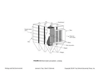
Schematic of wire-plate ESP • Introduction Fig.1 Schematic of wire-plate electrostatic precipitator
Mechanism of ESP • Introduction Fig. 2 Mechanism of electrostatic precipitator
Introduction 2.2.2 PROCESS OF Particle charging Particle charging is the first and foremost beginning in processes. As the voltageapplied on precipitator reach threshold value, the space inside divided into ionization region and drift region.
Introduction The electric field magnitude around the negative electrode is so strong that the electronsescape from molecule. Under the influence of electric field, the positive ions move towards the corona, while the negative ions and electrons towards the collecting plates.
Introduction 2.2.3 Particle transport In the moving way, under the influence of electric field, negative ions cohere and charge the particles, make the particles be forced towards collecting-plate as well as Fig.2 shows.
Introduction 2.2.4 Particle collection As soon as the particles reach the plate, they will be neutralized and packed by the succeeded ones subsequently. The continuous process happens, as a result, particles are collected on the collecting plate.
Research and design in ESP modeling The numerical model describes in time and space the relevant processes that are involved in transport, charging, migration and collection of fly ash. To represent the complete processes, the model is therefore structured into several modules.
The model here is organized into the following three sections: • electric field and discharge processes • particle charging • particle collection
3.1 electric field and discharge processes The particle collection in electrostatic precipitators is largely dominated by the distribution of the electric field in the interelectrodic space.
In the absence of particles, neglecting the transport gas velocity and by assuming that the magnetic field due to the corona current is negligibly small. Electronical conditions are described by next three equations :
Here V is the electric potential, is the space-charge density, is the permittivity of free space and E is the electric field. (1) (2) (3)
Here, we adopt equations (4) (5) (6) to describe the electric field distribution with the initial and boundary conditions.
V( x, y) means the electric potential of the position (x, y), V0 is the initial potential on the wire, Sx is distance between collecting plate and wire, Sy is half length of the two nearest wires ,a is the radius of particle, when x, y means the coordinates direction, shown as Fig.3.
(5) (6) and V0 mean the charge density and electric potential at the position as Fig.3 shown.
3.2 particle charging The field charging refers to the local distorsion caused near the particle surface by the difference in dielectric constants. This process continues until the particle goes up to the saturation charge, which produces an electric field on particle surface equal and opposite to the external field.
Equation (7) is chosen to describe the model of particle charging : (7) Where is the relative dielectric constant and E0 is the external field, qs and R are the particle charge and radius.
3.3 particle collection This module simulates in detail the boundary layer near the collecting plates and the interchange that take place. Here, we choose equation (8) to describe particle collection .
(8) C is the particle density, C0 is the entry density of particle, a is the unit collecting area in the flow way, f is area of ESP cross section, when w means particle velocity towards plate and v is the velocity moving to outlet.
4 Simulation results and analysis According the above analysis of the mechanism and modeling of ESP, we design a simple ESP simulation platform which is based on Scilab .
Simulation of electric field Fig.6 Distribution of electric field Ex
we can find that around the wires,Ex get a largest value, when at the connecting way of two wires, Ex is no more than zero. The cause of this distribution is the potential, at the connecting way of wires, nearly zero. Ex is decreased regularly from the wire at the coordinate line x, but larger when close to the collecting plate.
Simulation of electric field Fig.7 Distribution of electric field Ey
Simulation of particles density distribution Fig.8 Particle density distribution in ESP
From Fig.8, we see the particles density distribution obviously. The density reaches the largest value at the entry of the ESP under the influence of electric wind. The value of density gets smallest near the wire at the direction to collecting plate.
Simulation of deposit density Fig.9 Distribution of deposit density
Fig.9 shows us the deposit density, along the collecting plate deposit density is decreased definitely, since as time go on, the particle is collected by the plate continuously. So at the later part, the deposit density is lower, and reasonable.
CONCLUSION we construct a numerical model of electrostatic precipitator and design base on Scilab. The simulation resultsof these processes are according with laboratory experimental tests to obtain physical information and useful validations.
The End Thanks