Download
1 / 14
140 likes | 386 Vues
Macrostates and Microstates. A microstate is a particular configuration of the individual constituents of a system. A macrostate is a description of the conditions of the system from a macroscopic point of view. Let’s see two examples so this makes some sense.

E N D
Macrostates and Microstates A microstate is a particular configuration of the individual constituents of a system. A macrostate is a description of the conditions of the system from a macroscopic point of view. Let’s see two examples so this makes some sense. Example 1 – A gas: Consider 1 mol. of He gas at P = 1 atm and T = 298K. This is the macrostate of the gas – its condition described in terms of macroscopic parameters This gas has only one macrostate, if we change any of those macroscopic parameters, it’s a different macrostate. For each microstate, we’d have to fully describe the configuration of each of the 6.022 × 10²³ molecules. To do this we need to know its location (3 coordinates), velocity (3 coordinates) and time (1 coordinate for the whole system). A total of (6 × 6.022 × 1023) + 1 = 3.6 × 1024 coordinates. Note that a number of different microstates can have the same macrostate. The best way to realise this is to take our gas and move one of the atoms slightly – this is a new microstate as one of the microscopic parameters has changed, but the effect on the macroscopic parameters is infinitesimal, hence it’s the same macrostate. Thermal Physics
Macrostates and Microstates But it’s more interesting to see the relationship between micro- and macrostates the other way around. A gas in one particular macrostate could be in any of an infinite number of possible microstates. To give two out of an infinite number of examples – suppose I have a mixture of 14CO2 in 12CO2, one possible microstate has all of the 14CO2 in one corner of the volume, another has them evenly distributed throughout the gas. Both of these are the same macrostate, the gas has the same U,P,V,T,N, etc., but different microstates. Both are possible, so why is it we never see the first case and almost always see the second case? To answer that, we should look at the second example. PHYS 2060 Thermal Physics
Macrostates and Microstates Example 2 – Coin tossing: Let’s switch for a few moments to a system that’s a bit easier to handle (because there are only 8 configurations, not 1024). Let’s make it three coins, say a 1c coin, a 5c coin and a $2 coin (bronze, silver and gold, so that we can keep track of them easily). If we toss the three coins enough times, we’ll soon realise that there are 8 possible outcomes, which are shown in the table below. nheads = 3 (has 1 possible microstate) nheads = 2 (has 3 possible microstates) nheads = 1 (has 3 possible microstates) nheads = 0 (has 1 possible microstate) Each of the eight outcomes are our microstates, and we have four macrostates corresponding to the number of heads (nheads = 0, 1, 2 or 3) in our system. As you can see in the table, the macrostates with 0 and 3 heads have only one possible microstate, and the macrostates with 1 or 2 heads have three possible macrostates. PHYS 2060 Thermal Physics
Probability and Multiplicity The number of microstates corresponding to a given macrostate is called the multiplicity Ω of that macrostate, in the two cases above this is Ω (nheads = 0, 3) = 1 and Ω (nheads = 1, 2) = 3, respectively. Another point of note here is that if you know the microstate of a system then you know the macrostate of the system (for example, if it’s HHT then nheads = 2), but if you know the macrostate then you don’t necessarily know the microstate (for example, if nheads = 1, is it TTH, THT or HTT?). There is a lot of ‘information’ contained in a microstate. Let’s think a bit more about our coin example. The total multiplicity of all four possible macrostates is 1 + 3 + 3 + 1 = 8 = Ω(all), the total number of microstates. We can then write the probability of any particular microstate as: !(n) !(all) P(n heads) = (15.1) For example, P(2 heads) = Ω(2)/ Ω(all) = 3/8, which makes sense if you look back at the table above. PHYS 2060 Thermal Physics
Calculating the multiplicity Suppose we have 100 coins now, the total number of microstates is quite large: 2100, since each of the 100 coins has two possible states. The number of macrostates is 101: 0 heads, 1 head … up to 100 heads. What are the multiplicities of these macrostates? 0-heads: in this case, every coin lands tails up. Of course, there is only one possible microstate for this TTTTTTTT...TTTTTTTT, so Ω(0) = 1. 1-head: the heads-up coin could be in any one of 100 positions, so Ω(1) = 100. 2-heads: to find Ω(2), we need to think a little more carefully. You have 100 choices for the first coin, and for each of these choices you have 99 remaining choices for the second coin, but you could choose any pair in either order, so the number of distinct pairs is Ω(2) = (100 × 99)/2. 3-heads: here, you have 100 choices for the first, 99 for the second, 98 for the third, but any triplet can be chosen in several ways, 3 choices for the first flip and then 2 for the second flip, so the number of distinct triplets is Ω(3) = (100 × 99 × 98)/(3 × 2). PHYS 2060 Thermal Physics
Calculating the multiplicity By now, you can probably spot the pattern forming that will give us a general result. 100! &100 # n!(100 ' n)! % n " 100.99...(100 ' n + 1) n...2.1 = $$ !! ((n) = = (15.2) where n! is a factorial. We can take this one step further and arrive at a general expression for the multiplicity of a system with N-coins, which gives: N! & N # n!( N ' n)! % n ! = $$ ! (( N , n) = (15.3) " which is the number of ways of choosing n objects out of N. Lets just check this: Suppose we want the multiplicity for 2 coins in our 3 coin set. Ω(3,2) = 3!/[2!(3-2)!] = 6/[2*1] = 3, which is exactly as we’d expect. PHYS 2060 Thermal Physics
A physical example – the 1D spin chain • Finally, just to show this isn’t about coins, this can be applied directly to magnetic systems. For example, consider the 1-dimensional spin chain below. The multiplicity for any macrostate of this 1D spin chain is just: ) N & ( N" % N! N" !( N # N" )! N! N" ! N! ! '' $$ = *( N , N" ) = = (15.4) We can see that the maximum multiplicity will occur when N↑ = N↓, and later we’ll see that this corresponds to the state with the highest entropy. This is the very beginnings of a subject called statistical mechanics (PHYS3020), so I’ll leave this discussion here. PHYS 2060 Thermal Physics
Likelihood of macrostates, disorder & the 2nd law • Let’s go back to our coins. You’ll probably have noticed that if I take the three coins and throw them up in the air, that the macrostates nheads = 1 or 2 (probability 3/8ths each) are more likely than nheads = 0 or 3 (probability 1/8th each). And if I take 100 coins, I’m far more likely to get 49, 50 or 51 heads than get 0, 1, 99 or 100 heads. But in either case, if I choose any of the 8 or 1030 possible microstates, then they are all equally likely (probability 1/8 or 10−30 – 100-coins have 2100 ≈ 1030 microstates). So now you can probably spot a general rule here: The most likely macrostate for a system is the one with the largest number of microstates. Another thing you might have noticed with the coins is that the nheads = 0 or 3 macrostates are more ordered (i.e. are HHH or TTT) than the nheads = 1 or 2 macrostates (e.g HHT, HTH, TTH, etc), and that the more disordered macrostates (nheads = 1 or 2) are more likely, because they contain more microstates. This is because there are usually more ways of configuring the system if it’s got more disorder. Hence you could also say: The most likely macrostate of the system is the one with the most ‘disorder’. PHYS 2060 Thermal Physics
Evolution with time • Now lets consider how a system evolves with time, with our 100 coins, but this time we start with all coins as heads (one microstate). If each second, I randomly choose one coin and flip it at random, gradually the system evolves towards an equilibrium macrostate with ~ 50 heads and 50 tails organised at random (this macrostate has 100!/(50!50!) = 1029 microstates). This is a highly disordered state compared to our initial highly ordered ‘all heads’ microstate. If the system continues to evolve, it will fluctuate a bit (e.g., we may have 48 heads and 52 tails, sometimes), but we have to wait a long time to get all the heads back. Even if we were flipping all 100 coins each second, we’d expect to have to wait 1030s (or 1012 × the age of the universe) before we got ‘all heads’ back. For the moment you’ll need to trust that this idea translates across to other systems like gases, but already we can see a general rule emerging from our ‘coin’ system: Any large isolated system will spontaneously ‘evolve’ over time from non-equilibrium macrostates (those with a smaller number of microstates, lower multiplicity and low ‘disorder) towards equilibrium macrostates (those with the largest number of microstates, the highest multiplicity and the highest ‘disorder’). This is just a more general statement of the 2nd law. But where does entropy come into this? To resolve this, we need some work by Ludwig Boltzmann. PHYS 2060 Thermal Physics
Boltzmann’s entropy • Ludwig Boltzmann was an Austrian physicist working on the kinetic theory of gases in the late 1800s. His two main contributions were the velocity distribution of particles in a gas (i.e., the Maxwell-Boltzmann distribution) and the following connection between the microscopic properties of a system and its entropy. In fact, this latter result is what Boltzmann is best remembered for, and he felt it was so important that it be engraved on his tombstone. So what is this equation that we see written on Boltzmann’s tombstone? It is: S = k B ln ! or k B logW (15.5) where S is the entropy, kB = 1.38 × 10⁻²³ J/K is Boltzmann’s constant and W is the number of microstates corresponding to the macroscopic state of the system – this is just the multiplicity Ω that we developed earlier. Note that the log is an exponential/natural log (or ln) not a base 10 log. PHYS 2060 Thermal Physics
Boltzmann’s version of the 2nd law So what is this equation that we see written on Boltzmann’s tombstone? It is: S = k B ln ! or k B ln W (15.5) where S is the entropy, kB = 1.38 × 10⁻²³ J/K is Boltzmann’s constant and W is the number of microstates corresponding to the macroscopic state of the system – this is just the multiplicity Ω that we developed earlier. Note that the log is an exponential/natural log (or ln) not a base 10 log. If we apply Boltzmann’s law to the general result we just arrived at, we obtain: Any large isolated system in equilibrium will be found in the macrostate with the greatest entropy (aside from fluctuations normally too small to measure), and non- equilibrium systems with lower entropy will spontaneously evolve towards this maximally-entropic, equilibrium state. This is something known as the entropic statement of the 2nd law or the principle of increase in entropy (some will also call it Boltzmann’s statement of the 2nd law). PHYS 2060 Thermal Physics
Horribly Large Numbers!! The standard entropy for a mole of ice ΔS0 at 273K is 41 J/K, let’s follow this through the Boltzmann equation. So, ln Ω = ΔS0/kB = 41/1.38×10-23 = 2.9×1024 giving log10 Ω = 0.43 × 2.9×1024 = 1.3×1024 and so Ω = 101.3×10^24 = 101,300,000,000,000,000,000,000,000!!!! This is a HUGE number, for example, there are only about 1070 particles in the entire universe. Now if we consider water at 273K, then ΔS0 = 63 J/K, and this gives a larger Ω = 102,000,000,000,000,000,000,000,000, this is bigger, but not to a massive extent. With these sorts of numbers in mind, any idea of ‘order’ and ‘disorder’ goes out the window. Be really careful with these two terms – they work great as a way to get the concept, but they are actually wrong, and so once you understand it, they are best abandoned for other descriptions of entropy. PHYS 2060 Thermal Physics
An unlikely arrangement • Suppose we have a gas in a box, how long would we have to wait for it to end up in a microstate where all of the gas is in one half of the box, as shown to the right. Note this is equivalent in the 100-coin system to a macrostate with 100 heads and 0 tails, which is very rare because it’s the most ordered of ~1030 possible microstates. This might seem like we’re stretching the coin analogy too far, but its not. If we wanted to, we could just represent this system with L = particle in the left side and R = particle in the right side, instead of H and T – it’s exactly the same as the coins! What we’re doing is to effectively halve the volume of the gas. If we look at Eqn. 20.6, replacing V by V/2 reduces the multiplicity by a factor of 2N. In other words, the probability of all the molecules being on the left is 2−N. For N = 100, this probability is ~10−29, and you would have to check a trillion times a second for the age of the universe before finding such an arrangement once. For ~1 mol. of a gas, N ~ 1023 and so the probability might is infinitesimally small and we can fairly safely expect to never see a gas occupying half a volume. PHYS 2060 Thermal Physics
Summary • • • • • While entropy can be described macroscopically as the ratio Q/T, it also has a microscopic description. A microstate is a particular configuration of the individual constituents of a system. A macrostate is a description of the conditions of the system from a macroscopic viewpoint. A system can have a number of possible macrostates, each with its own microstates. A number of different microstates can have the same macrostate, and a macrostate can have anything from one to an infinite number of microstates. Based purely on probability, it is possible to say that the most likely macrostate for a system is the one with the largest number of microstates. Boltzmann’s law relates entropy to the multiplicity of microstates of a system via S = kBlnΩ. This results in the entropic statement of the 2nd law (or principle of increasing entropy) which states that any large system in equilibrium will be found in the macrostate with the greatest entropy (aside from small fluctuations). In the next lecture we will look at the second law from the macroscopic viewpoint of entropy and try to link the two pictures together. PHYS 2060 Thermal Physics