Download
1 / 32
340 likes | 533 Vues
Intensity interferometry for imaging dark objects. Dmitry Strekalov , Baris Erkmen , Igor Kulikov , Nan Yu. Jet Propulsion Laboratory, California Institute of Technology Quantum Sciences and Technology group. Ghost Imaging with thermal light. Theory: Experiment:. Object. Image.

E N D
Intensity interferometry for imaging darkobjects Dmitry Strekalov, BarisErkmen, Igor Kulikov, Nan Yu Jet Propulsion Laboratory, California Institute of Technology Quantum Sciences and Technology group
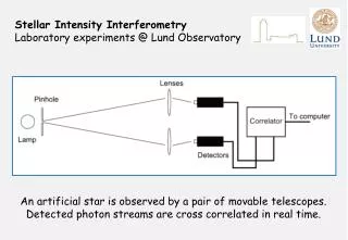
Ghost Imaging with thermal light Theory: Experiment: Object Image 50/50 beam splitter Transverse mode (speckle) size
Can an object replace the beam splitter? x' x1 Object Image x2
This enables two possible observation scenarios Source Source Object Object
Our model and approach Key assumptions: • Paraxial approximation • Flat source and object • Gaussian distribution • of source luminosity • and object opacity [D.V. Strekalov, B.I. Erkmen, and N. Yu, Phys. Rev. A, 88, 053837 (2013)]
Gaussian absorber on the line of sight Speckle width Ro = 1, 2, 3 mm 50 cm r Rs = 1 cm r 50 cm A small absorbing object has little effect on the speckle shape, but affects its width.
Gaussian absorber crossing line of sight Parallel Perpendicular 9% 9% 6% 50 cm r Rs = 1 cm r 50 cm Ro = 1 mm Transition direction matters! “Stereoscopic vision”
Source: Rs = 0.94R , Ls= 12 Rs, angular size 1.5e-10 radians Object: Ro = REarth, L = 290 pc, angular size 1.2e-12 radians Kepler 20e, intensity measurement Object appears smaller than the source; speckle smaller than the object; speckle smallerthan the shadow 1.9 10-4 x Francoiset al. Nature 482 195-198 (2012)
Kepler 20e, speckle width measurement (hypothetical) 1+5.5 10-5 1-1.1 10-4 1.7 10-4 x x x 1 Max fractional width variation Detectors base We could determine the transient direction!
What SNR should we expect from a real thermal light source? Broadband detectionNarrow-band detection Full optical bandwidth and power of the source; g(2)contrast reduced due to multimode detection. Reduced optical bandwidth and power of the source; full contrast of g(2)due to single-mode detection. WBdetection bandwidth T0 coherence time T integration time Table-top pseudo- thermal Astronomy stellar In the low spectral brightness regime (e.g., faint black body radiation), these two scenarios yield similar SNR. For spectrally resolved observation (e.g., a specific atomic transition), narrowband detection provides an advantage! In any case, large WBis beneficial. [D.V. Strekalov, B.I. Erkmen, and N. Yu, Phys. Rev. A, 88, 053837 (2013)]
How is the object’s signature encoded in the correlation function source If the source speckle upon the object is smaller than the object feature, Introducing and (symmetric configuration) or approximately (large source, small object) Fourier-transform of the source luminosity (van Cittert–Zernike theorem) The source luminosity Fourier-transform of the object opacity
Gerchberg-Saxton algorithm for dark objects FT FT-1 Correlation function (observed) Corfunction constraint Object constraint Object’s profile (reconstructed) Correlation function constraint: the absolute value must match the observation Object absorption constraint: 1. A is Real 2. 0<A<1* 3. Size limitation (not expected to be larger than…) 4. Often we know that the object is solid: A = 0 orA = 1* 5. Using low-resolution “support” image *) These constraint are specific to our approach
Image reconstruction example (numerical simulation on the lab scale) Source: R = 2 mm, l = 532 nm, Gaussian luminosity distribution Detectors array to measure the correlation function 36 cm Object 36 cm • In this geometry, the object produces no tell-tale shadow! 2 mm X 1000 brightness amplification 6.4 mm 6.4 mm The source speckle observed in the correlation function measurement (on the left) is modified by the presence of the object. By artificially increasing its brightness (on the right) we can clearly see a structure encoding the spatial distribution of the object’s opacity, which is to be recovered.
The reconstruction results (not using the “solid object” A = 0 orA = 1 constraint) [D.V. Strekalov, I. Kulikov, and N. Yu, to appear in Optics Express (2014)]
Handling solid (A= 0 orA = 1) objects 1 1 1 0.5 0 0 0 1 0.5 0.5 1 1
Astrophysics example: a hypothetical Earth-size planet in the Oort cloud Sirius 8.6 ly 1 ly arc sec arc sec with two 1000 km moons 0.7 % flux reduction Detectors array: 2000 x 2000, 1m-spaced, 532 nm Detectors array are so large in order to capture the source speckle and the object/pixel speckle at the same time. Can we avoid insanely large arrays?
The reconstruction results Iteration # 0 (initial guess) 1 10 20 Iteration # 30 40 50 60 Iteration # 70 80 90 100
Experimental demonstration with a pseudo-thermal light source Correlation observable: Ixy Iyx
Experiment 1. Double slit Rs= 2.15 mm Gaussian spot 60 cm 90 cm Ix I-x Slits width 0.22 mm, distance between centers 1.01 mm X (mm)
Experiment 2. Double wire Rs= 2.15 mm Gaussian spot 58 cm 89 cm Wires diameter 0.32 mm, distance between centers 1.4 mm X (mm)
There are many phase objects in space! (Gravitational lensing and microlensing) The Einstein Cross: four images of a distant quasar Q2237+030appear due to strong gravitational lensing caused by a foreground galaxy. Photo by Hubble. A luminous red galaxy (LRG 3-757) has gravitationally distorted the light from a much more distant blue galaxy. Photo by Hubble.
Intensity-interferometric imaging of a phase object isn’t good enough; need higher-order terms Phase contribution Example: a parabolic lens ; Where Is[…] is the intensity of the source, and is the gradient of phase. when Is[…] =Is[0] = const, and
Use Gerchberg-Saxon algorithm to recover the source function with modified argument Invert Is[…] to recover Keep this piece, remove the rest of the lens Phase object reconstruction steps: 50 cm 50 cm f = 11.36 cm Encoding into Restoring after correlation function 500 iterations Original phase object cm cm Restored phase object
Summary A dark object in the line of sight affects a light source correlation function, imprinting upon it its own optical properties. This phenomenon may be used for intensity-interferometric imaging of this object. This technique may be promising for high-resolution observation of a variety of space objects and phenomena, e.g. • Exoplanets • Neutron stars • Kuiper Belt / Oort cloud objects • Dark matter • Gas or dust clouds • Gravitational lensing and microlensing SNR in the intensity-interferometric imaging of dark objects is not favorable but may be suitable in narrow-bandwidth measurements.
The UMBC Ghost Imaging experiment UMBC (photon energy conservation) f b a1 Photon pairs source (photon momentum conservation) (x,y) a2 • Background suppression • Imaging of difficult to access objects • Dual-band imaging • Relaxed requirements on imaging optics
Statistics of photon detections Glauber correlation function Laser light: g(2)(0) = 1 Poisson statistics (random process) Pulsed light: g(2)(0) > 1 “Bunching” Amplitude-squeezed light: g(2)(0) < 1 “Anti-bunching” (quantum!) Single-mode thermal light:g(2)(0) = 2 “Bunching” “UR” “UMBC” ???
Two-coordinate correlation function can be introduced likewise x1 x2 Observed by means of photodetectionscoincidences. In practice, one measures with single-photon measurements, or with photocurrents measurements
Phase objects models for Gravitational Lensing Gravity plane grad f a Source Detector where We consider three common* models for mass distribution: Gravity plane of constant surface mass-density Σ=const. This model corresponds to the constant mass distribution of the matter near the symmetry axis. The surface mass-density of the plane Σ ~ 1/ξ. This model is a simple realization of spatial distribution of matter in galaxies, clusters of galaxies, etc. A point mass. This model corresponds to a black hole or another very compact space object. *) “A Catalog of Mass Models for Gravitational Lensing”, arXiv:astro-ph/0102341v2
(0) Free-space propagation. Gravity plane of constant surface mass-density Σ=const. where the modified length L*depends on the surface mass density. This is equivalent to free-space propagation over a greater distance. (b) The surface mass-density of the plane is inversely proportional to impact parameter ξ. where d0 depends on the total mass. This multiplies the correlation function by an unobservable phase factor. The off-axis configuration may lead to observable effects and needs to be analyzed.
The cost of narrow-band detection 1 ps timing resolution 3.3 nm bandwidth @ l = 1 mm. Loss relative to maximally wide-band intensity measurement is 23 dB (again, much less for a color-resolved measurement)
Kuiper Belt 30-50 AU from the Sun. Roques F., et al., Astron. J., 132, 819–822 (2006): Chang H., et al.,Nature, 442, 660–663(2006):