Download
1 / 44
440 likes | 573 Vues
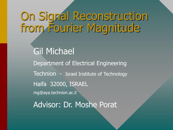
On Signal Reconstruction from Fourier Magnitude. Gil Michael Department of Electrical Engineering Technion - Israel Institute of Technology Haifa 32000, ISRAEL mg@aya.technion.ac.il Advisor: Dr. Moshe Porat. Lecture Outline. Introduction to Fourier Magnitude Reconstruction

E N D
On Signal Reconstruction from Fourier Magnitude Gil Michael Department of Electrical Engineering Technion - Israel Institute of Technology Haifa 32000, ISRAEL mg@aya.technion.ac.il Advisor: Dr. Moshe Porat
Lecture Outline • Introduction to Fourier Magnitude Reconstruction • Fourier Magnitude Applications • Reconstruction by Decimation-in-Time FFT • Reconstruction from Local Fourier Magnitudes • The Intermediate Fourier-Domain Algorithm (IFD) • Summary and Discussion
Introduction • Reconstruction of signals from their Fourier transform properties is a useful task in science and engineering. • Fourier transform properties consist of phase and magnitude information:
Introduction - Cont’d (2) • Discrete Fourier Transform (DFT) notation 1-D: 2-D:
Reconstruction from Fourier Magnitude or Phase Original Magnitude Phase DFT IDFT IDFT
Introduction - Cont’d (3) The Fourier phase contains higher intelligibility than Fourier magnitude BUT Fourier phase is more difficult to obtain
Applications of Reconstruction from Fourier Magnitude Spectroscopy After: A.Yariv,Optical Electronics
Applications of Reconstruction from Fourier Magnitude Diffraction Pattern
Applications of Reconstruction from Fourier Magnitude-Cont’d Crystallography After:Ramachandran & Srinivasan,Fourier Methods in Crystallography
Reconstruction from Fourier Magnitude - Limitations Global Fourier magnitude is, in general, insufficient information for reconstruction Additional data is required: Spatial data, finite support, FT Sign- information, localized Fourier magnitude
Algorithm I Reconstruction by Decimation-in-Time FFT From Nawab et al. (1983) we know, that a sequence x(n), which is zero outside 0nN-1, is uniquely specified by its spectral magnitude and at least N/2 samples of x(n). The proof relies on the relationship between the Fourier magnitude and the auto-correlation function. The proposed algorithm is a closed-form solution to a similar problem:
Reconstruction by Decimation-in-Time FFT (Cont’d) Given the Fourier magnitude of a real signal x(n), which is zero outside 0nN-1, and the even (odd) samples, find a closed-form solution to the odd (even) unknown samples. • Use the Decimation-in-Time FFT algorithm * We will assume N is a power of 2, such that N=2L for some integer L>0
Decimation-in-Time FFT After: Cooley & Tukey, 1965
Decimation-in-Time FFT (Cont’d) The problem of finding xodd [n] is equivalent to retrieving the N/2-point DFT values of xodd [n]: (1)
Decimation-in-Time FFT - Detail We may write the squared magnitude as: (a) (b)
Decimation-in-Time FFT - Detail And we obtain the absolute value of H[k] from: (c) For the retrieval of the phase qHKwe rewrite X[k] in the polar form:
Decimation-in-Time FFT - Detail (d) Summing and subtracting (d) and applying DFT properties of real signals, (e)
Decimation-in-Time FFT - Detail Adding the square products of (e), (f) And the resulting phase,
Decimation-in-Time FFT (Cont’d) (2) (3)
Decimation-in-Time FFT (Cont’d) Ambiguity in the phase of H[k] is resolved by using the interpolate by 2 formula: (4)
Decimation-in-Time FFT: Extension to 2-D signals (Images) An image may be fully reconstructed using the Decimation-in-Time FFT approach, with some constraints imposed on it. The even rows (columns) must be symmetric i.e., in each even row (column), x(m,n)=x(N-m,n). The 2-D Fourier magnitude of x(m,n) and the 1-D Fourier magnitude of the even rows (columns) are known.
Decimation-in-Time FFT: The Intermediate Fourier Domain The 2-D DFT may be implemented by an FFT on the image’s rows (columns) and then on the resultant columns (rows). The intermediate Fourier domain (IFD) is defined as the resultant matrix obtained after the first row (column) FFT.
Decimation-in-Time FFT: Extension to 2-D signals (Cont’d) • Since the rows (columns) are symmetric, their (1-D) Fourier transforms are real. In addition: • The columns (rows) of the image’s Fourier- transform are the (1-D) Fourier transforms of the IFD columns (rows).
Decimation-in-Time FFT : Intermediate Fourier Domain Example DFT Rows Columns DFT Performed On Columns
Decimation-in-Time FFT: Extension to 2-D signals (Cont’d) • Using the Decimation-in-Time FFT algorithm, reconstruct the image from: 1) The calculated even (odd) samples of the IFD columns 2) Fourier transform magnitude of the image
Algorithm II Reconstruction from Local Fourier Magnitudes Recently, it was found that an image is represented by its Fourier magnitude and a quarter of its spatial samples (Shapiro & Porat, 1998) However, spatial samples may not always be available. In the following algorithm, image reconstruction from local Fourier magnitudes requires only a single spatial sample.
Reconstruction from Local Fourier Magnitudes - Cont’d Local Fourier magnitudes are the absolute values of Fourier transforms taken over specific sections of the image. Two methods of reconstructing an image from local Fourier magnitudes and a single spatial sample are presented here. In addition it is shown, that reconstruction quality is relatively unaffected by spatial data errors.
Reconstruction from Local Fourier Magnitudes - Cont’d The first algorithm is based on successively reconstructing larger and larger image blocks, with each newly reconstructed block being the spatial samples required for the next iteration. The second algorithm, iteratively reconstructs equal-sized blocks that overlap by ¼ of their samples.
Local Fourier magnitudes – Successive Block-Size Reconstruction Algorithm
Local Fourier magnitudes Reconstruction Algorithm– Successively larger Image Blocks method Known Spatial Block
Local Fourier magnitudes Reconstruction Algorithm– Overlapping Equal-Sized Blocks method (32x32 pixels) Known Spatial Block
Reconstruction from Local Fourier Magnitudes and an Arbitrary Spatial Sample Note: inconsistency Reconstructed Original
Algorithm III The Intermediate Fourier- Domain Reconstruction Algorithm Gerchberg-Saxton algorithm: iteratively imposes spatial constraints, known samples and Fourier magnitude in the spatial and Fourier domains As shown previously, the 2-D DFT may be implemented using the Intermediate Fourier Domain (IFD).
The Intermediate Fourier-Domain Reconstruction Algorithm - Cont’d A typical reconstruction scheme would require a 2N x 2N DFT for an N x N image, essentially zero-padding the additional spatial samples:
The Intermediate Fourier-Domain Reconstruction Algorithm - Cont’d • The IFD, preserves some of the spatial constraints: • Finite support. • Nulling of the columns (rows) of the result.
The Intermediate Fourier-Domain Reconstruction Algorithm - Cont’d The proposed algorithm utilizes these properties to modify the Gerchberg-Saxton approach. It uses 1-D FFT’s only, and imposes twice as many magnitude constraints in each iteration, resulting in faster convergence to the desired image.
Intermediate Fourier-Domain Algorithm: Iterative Simulation Iteration: 6 4 5 8 10 1 2 3 9 7 25% known spatial samples
Intermediate Fourier-Domain Algorithm: Comparison After 10 Iterations
Intermediate Fourier-Domain Algorithm: Simulation Results After 100 Iterations 18dB
Summary • Three new approaches to signal reconstruction from Fourier magnitude were presented. I) Decimation-in-Time FFT Algorithm: • Closed-form solution: No iterations and convergence uncertainty. • Lower computational complexity compared to the auto-correlation approach. • Efficient implementation (FFT). • 2-D Extension requires only Fourier information.
Summary - Cont’d II) Localized Fourier Transform Magnitude Algorithm: • Magnitude information and a single spatial sample fully reconstruct the image. • Two methods may be applied: constant block or successively larger block reconstruction. • This algorithm may prove useful in phase retrieval problems, where spatial information is unavailable (in contrast to Nawab et al.).
Summary - Cont’d III) Intermediate Fourier Domain Algorithm • A modified Gerchberg-Saxton algorithm utilizes the separability property of the 2-D DFT. • Imposes the Fourier magnitude constraints at twice the rate of the conventional approach, resulting in faster convergence rates.