Download
1 / 32
440 likes | 1.07k Vues
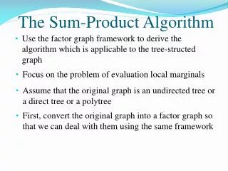
The Sum-Product Algorithm. Use the factor graph framework to derive the algorithm which is applicable to the tree- structed graph. Focus on the problem of evaluation local marginals. Assume that the original graph is an undirected tree or a direct tree or a polytree.

E N D
The Sum-Product Algorithm • Use the factor graph framework to derive the algorithm which is applicable to the tree-structed graph • Focus on the problem of evaluation local marginals • Assume that the original graph is an undirected tree or a direct tree or a polytree • First, convert the original graph into a factor graph so that we can deal with them using the same framework
Goal • The goal is to exploit the structure of the graph to achieve the two thing: (i) To obtain an efficient, exact inference algorithm for finding marginals (ii) In situations where several marginals are required to allow computations to be shared efficiently
The Sum-Product Algorithm • Suppose that all of the variables are hidden • By definition, Joint distribution The set of variables in x without including x • Use • Then, interchange the summations and the product
The Sum-Product Algorithm • Consider the following graph Joint distribution The product of all the factors in the group associated with factor
The Sum-Product Algorithm • Substitution into and interchanging the sums and products • Introduce a set of functions: • View as messages from the factor node to the variable node x
The Sum-Product Algorithm Denoted • Each factor is described by a factor (sub-)graph and so can itself be factorized.
The Sum-Product Algorithm The message that go from factor nodes to variable nodes The message that go from factor nodes to variable nodes
The Sum-Product Algorithm • Derive an expression of evaluating the message from variable nodes to factor nodes, again by making the sub-graph factorization
The Sum-Product Algorithm • Each of these message can be computed recursively in term of messages • To start the recursion, view the node x as the root of the tree and begin at the leaf nodes • If a leaf node is a variable node, then the message that is sent along its one and only one link • If the leaf node is a factor node, the message should take the form
The Sum-Product Algorithm • Start by viewing the variable node x as the root of the factor graph and initiating messages at the leave • The message passing steps are then applied until messages have been propagated along every link • The root node will receive messages from all its neighbours • The required marginal can be evaluated
Example • Unnormalized joint distribution: Root leaf
Sum-Product And Max-Sum Algorithm • Sum-product algorithm: • Take a joint distribution expressed as a factor graph • Efficiently find marginals over the component variables • Max-sum algorithm: • Find a setting of the variables that has the largest probability • Find the value of the above probability • Viewed as an application of dynamic programming
Find the maximal value • Run the sum-product algorithm to obtain for every variable, and then, for each marginal in turn, to find the value that the maximizes the marginal • Or, find the set of values that have the largest probability, we can find the vector that the maximizes the joint distribution • However, the is not always the same as the set of
Example Max • So, the marignals are maximized by and , which corresponds to a value of 0.3 Max • But, the largest joint probability is 0.4
The Max-Sum Algorithm • Write out the max operator: where M is the total number of variables • Substitute for using the product of factors and use the distributive law of multiplication
The Max-Sum Algorithm • The final maximization is performed over the product of all messages arriving at the root node, and gives the maximum value for • This is called the max-product algorithm and identical to the sum-product algorithm except that summations are replaced by maximization
The Max-Sum Algorithm • Product of many small probabilities can lead to numerical underflow problem, so work with the logarithm of the joint distribution • If then • The logarithm function makes the products be the sums, so we can obtain the max-sum algorithm
The Max-Sum Algorithm • The initial message: • The probability at the root node:
The Max-Sum Algorithm • Finding the maximum of the joint distribution is irrespective of which node is chosen as the root • The process of evaluating the above equation will give the value for the most probable value of the root variable
The Max-Sum Algorithm …. …. 144 The simple chain with N variables each having K states Take the as the root node In the first phase, propagate messages from the leaf node to the root node using The initial message: The most probable value for is given by
The Max-Sum Algorithm • Need to determine the state of previous variables that correspond to the same maximizing configuration • Done by keeping track of which values of the variables gave rise to the maximum state of each variable
The Max-Sum Algorithm Lattice or trellis diagram The variable node The nodes with the second states • Not a probabilistic graphical because the nodes represent individual states of variable • For each state of a given variable, there is a unique state of the previous variable that maximizes the probability, corresponding to the function , and indicated by the line connecting the node
The Max-Sum Algorithm • Once, we know the most probable value of the final node , simply follow link back to find the most probable state of node and so back to the initial node • Using and is known as back-tracking
The Max-Sum Algorithm • Two paths, each of which we shall suppose corresponds to a global maximum
The Max-Sum Algorithm • If a message is sent from a factor node f to a variable node x, a maximization is performed over all other variable node that neighbours of that factor nodes, using • Performing this maximization, keep recode of which values of the variables gave rise to the maximization • In the back-tracking step, having found , then use these stored values to assign consistent maximizing states