Download
1 / 25
250 likes | 375 Vues
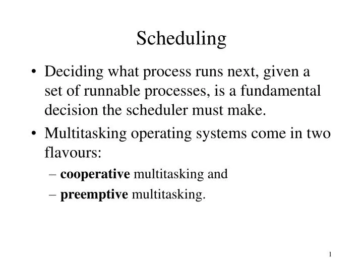
Scheduling. Deciding what process runs next, given a set of runnable processes, is a fundamental decision the scheduler must make. Multitasking operating systems come in two flavours: cooperative multitasking and preemptive multitasking.

E N D
Scheduling • Deciding what process runs next, given a set of runnable processes, is a fundamental decision the scheduler must make. • Multitasking operating systems come in two flavours: • cooperative multitasking and • preemptive multitasking.
The act of involuntarily suspending a running process is called preemption. The time a process runs before it is preempted is predetermined, and is called the timeslice of the process. • In cooperative multitasking, a process does not stop running until it voluntary decides to do so. The act of a process voluntarily suspending itself is called yielding. Problems: • The scheduler cannot make global decisions on how long processes run, processes can monopolise the processor for longer than the user desires, and a hung process that never yields can potentially bring down the entire system.
Policy - determines what runs when and is responsible for optimally utilising processor time. • I/O-Bound Versus Processor-Bound Processes • I/O bound spends much of its time submitting and waiting on I/O requests. • Processor-bound processes spend much of their time executing code. They tend to run until they are preempted as they do not block on I/O requests very often. • Sheduling policy must attempt to satisfy two conflicting goals: fast process response time (low latency) and high process throughput. • Favouring I/O-bound processes provides improved process response time, because interactive processes tend to be I/O-bound. • To provide good interactive response, Linux optimises for process response (low latency), thus favouring I/O-bound processes over processor-bound processors.
Timeslice • The timeslice is the numeric value that represents how long a task can run until it is preempted. • A timeslice that is too long will cause the system to have poor interactive performance. • A timeslice that is too short will cause significant amounts of processor time to be wasted on the overhead of switching processes • I/O-bound processes do not need longer timeslices, whereas processor-bound processes crave long timeslices • It would seem that any long timeslice would result in poor interactive performance. • The Linux scheduler dynamically determines the timeslice of a process based on priority. This enables higher priority, allegedly more important, processes to run longer and more often.
A process does not have to use all its timeslice at once. For example, a process with a 100 millisecond timeslice does not have to run for 100 milliseconds in one go instead, it could can run on five different reschedules for 20 milliseconds each.
Scheduling criteria • CPU utilisation – 40% to 90% • Throughput – number of processes completed in a given time • Turnaround time – time from submission to completion • Waiting time – sum of the periods waiting in ready queue • Response time – time to start responding
First Come First Served • This is a non pre-emptive scheme – runs to completion if no I/O • Not usually used on its own but in conjunction with other methods • This scheme was used by Windows up to version 3.11 • The average waiting time for the above example is • (0 + 2 +62 + 63 + 66)/5 = 38.6
Shortest Job First (SJF) • Non pre-emptive • What is the length of the next process? • Prediction • The average waiting time for the above example is • (0 + 1 + 3 + 6 + 56)/5 = 13.2
Shortest Job First (SJF) • Non pre-emptive • What is the length of the next process? • Prediction • The average waiting time for the above example is • (0 + 1 + 3 + 6 + 56)/5 = 13.2
Priority Scheduling e.g. SJF where priority is inverse of the next CPU burst • Indefinite blocking or starvation – leaves low priority • processes waiting forever • Ageing 0 1 6 16 18 19
Ageing PID priority A Finishes time slice, priority reset 15 The queue is then aged A becomes current again A’s priority reset A 15 Inserts after next lowest number B 15
Ageing (cont) B Finishes time slice, priority reset 14 F 12 Queue is aged And so on! Note that ‘F’ eventually reaches the Front of the queue.
Round Robin Scheduling • Each process gets a ‘time quantum’ or ‘time slice’ • Processes kept in a FIFO buffer if process < 1 time quantum completes else interrupt causes context switch • Average waiting time = 0 + 4 + 7 + 6= 17/3 = 5.66ms • If times are short context switching causes an overhead.
Multi-level Queue Scheduling • Foreground processes – interactive • Background processes Highest priority System processes Interactive processes Interactive editing processes Batch processes Student processes Lowest priority • Multi-level Feedback Queue Scheduling • Allows movement up and down into different queues
Linux • Uses MFQ with 32 levels • Each queue uses round robin scheduling with ageing • User can alter priorities using the ‘nice’ command Real Time Linux • Kernel processes are non preemptive • Interrupts disabled in critical sections of code • Real time code swapped out
Real-time Operating Systems • Definition: A real-time operating system (RTOS) is an operating system that guarantees a certain capability within a specified time constraint. • Hard real-time tasks are required to meet all deadlines for every instance, and for these activities the failure to meet even a single deadline is considered catastrophic. Examples are found in flight navigation, automobile, and spacecraft systems. • Soft real-time tasks allow for a statistical bound on the number of deadlines missed, or on the allowable lateness of completing processing for an instance in relation to a deadline. Soft real-time applications include media streaming in distributed systems and non-mission-critical tasks in control systems. • Periodic Real-time Tasks - is a task that requests resources at time values representing a periodic function. That is, there is a continuous and deterministic pattern of time intervals between requests of a resource. In addition to this requirement, a real-time periodic task must complete processing by a specified deadline relative to the time that it acquires the processor (or some other resource). • For example, a robotics application may consist of a number of periodic real-time tasks. Suppose the robot runs a task that must collect infrared sensor data to determine if a barrier is nearby at regular time intervals. If the configuration of this task requires that every 5 milliseconds it must complete 2 milliseconds of collecting and processing the sensor data, then the task is a periodic real-time task.
Aperiodic real-time tasks involve real-time activities that request a resource during non-deterministic request periods. Each task instance is also associated with a specified deadline, which represents the time necessary for it to complete its execution. • Examples of aperiodic real-time tasks are found in event-driven real-time systems, such as ejection of a pilot seat when the command is given to the navigation system in a jet fighter. As in normal operating systems schedulers can be classified as preemptive and priority based. • They can be a combination of strategies (e.g., preemptive prioritised). • It is perfectly reasonable to have a prioritised, non-preemptive (e.g. run to completion) scheduler. • Prioritised-preemptive schedulers are the most frequently used in RTOSs.
Fixed-priority scheduling algorithms do not modify a job's priority while the task is running. The scheduler is fast and predictable with this approach. The scheduling is mostly done offline (before the system runs). This requires the system designer to know the task set a-priori (ahead of time) and is not suitable for tasks that are created dynamically during run time. The priority of the task set must be determined beforehand and cannot change when the system runs unless the task itself changes its own priority. • Dynamic scheduling algorithms allow a scheduler to modify a job's priority based on one of several scheduling algorithms or policies. This is a more complicated and leads to more overhead in managing a task set in a system because the scheduler must now spend more time dynamically sorting through the system task set and prioritising tasks. The active task set changes dynamically as the system runs. The priority of the tasks can also change dynamically.
Static Scheduling Policies • Rate-monotonic scheduling(RMS)Rate monotonic scheduling is an optimal fixed-priority policy where the higher the frequency (1/period) of a task, the higher is its priority. Rate monotonic scheduling assumes that the deadline of a periodic task is the same as its period. • Deadline-monotonic schedulingDeadline monotonic scheduling is a generalisation of the RMS. In this approach, the deadline of a task is a fixed (relative) point in time from the beginning of the period. The shorter this (fixed) deadline, the higher the priority.
Example 1 shows a single periodic task where the task t is executed with a periodicity of time t. • Example 2 adds a second task S where its periodicity is longer than that of task t. The task priority shown is with task S having highest priority. In this case, the RMS policy has not been followed because the longest task has been given a higher priority than the shortest task. However, in this case the system works fine because of the timing of the tasks periods • Example 3 shows the problems if the timing is changed, when t3 occurs, task t is activated and starts to run. It does not complete because S2 occurs and task S is swapped-in due to its higher priority. When task S completes, task t resumes but during its execution, the event t4 occurs and thus task t as failed to meet its task 3 deadline. This could result in missed or corrupted data, for example. When task t completes, it is then reactivated to cope with t4 event. • Example 4 shows the same scenario with the task priorities reversed so that task t pre-empts task S. In this case, RMS policy has been followed and the system works fine with both tasks reaching their deadlines.
Dynamic Scheduling Policies - can be broken into two main classes of algorithms. The dynamic planning based approach This approach is very useful for systems that must dynamically accept new tasks into the system; After a task arrives, but before its execution begins, a check is made to determine whether a schedule can be created and handled. Another approach, called the dynamic best effort approach, uses the task deadlines to set the priorities. With this approach, a task could be pre-empted at any time during its execution. So, until the deadline arrives or the task finishes execution, we do not have a guarantee that a timing constraint can be met. • Dynamic priority preemptive scheduling (dynamic planning approach) - the priority of a task can change from instance to instance or within the execution of an instance. A higher priority task preempts a lower priority task. Very few commercial RTOS support such policies because this approach leads to systems that are hard to analyse. • Earliest deadline first scheduling (dynamic best effort ) Earliest deadline first scheduling is a dynamic priority preemptive policy. With this approach, the deadline of a task instance is the absolute point in time by which the instance must complete. The task deadline is computed when created. The operating system scheduler picks the task with the earliest deadline to run. A task with an earlier deadline preempts a task with a later deadline. • Least slack scheduling (dynamic best effort )Least slack scheduling is also a dynamic priority preemptive policy. The slack of a task instance is the absolute deadline minus the remaining execution time for the instance to complete. The OS scheduler picks the task with the shortest slack to run first. A task with a smaller slack preempts a task with a larger slack. This approach maximises the minimum lateness of tasks.
Dynamic vs. Static Scheduling Using the Deadline Monotonic approach