Download
1 / 25
250 likes | 424 Vues
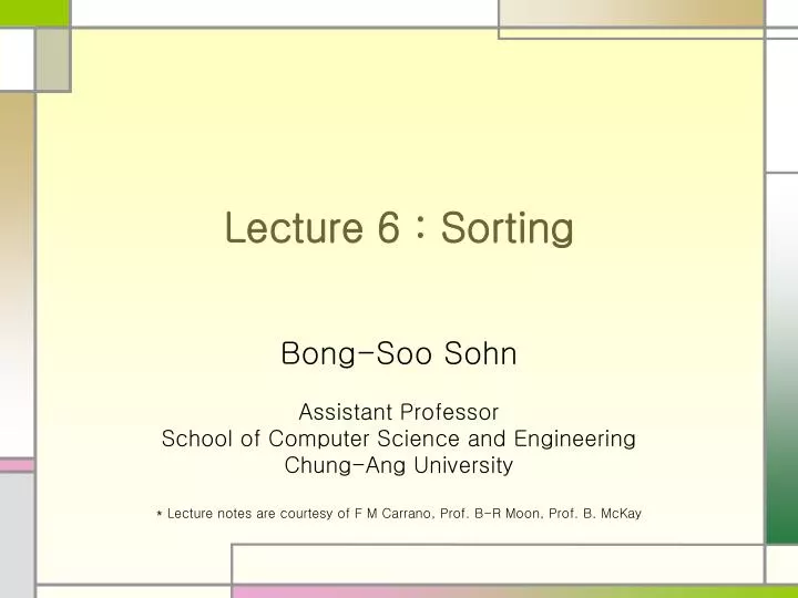
Lecture 6 : Sorting. Bong-Soo Sohn Assistant Professor School of Computer Science and Engineering Chung-Ang University * Lecture notes are courtesy of F M Carrano, Prof. B-R Moon, Prof. B. McKay. Sorting and Efficiency. Efficiency Big O Notation Worst, best and average case performance

E N D
Lecture 6 : Sorting Bong-Soo Sohn Assistant Professor School of Computer Science and Engineering Chung-Ang University * Lecture notes are courtesy of F M Carrano, Prof. B-R Moon, Prof. B. McKay
Sorting and Efficiency • Efficiency • Big O Notation • Worst, best and average case performance • Simple sorting algorithms • Selection sort • Bubblesort • Insertion Sort • Partitioning Algorithms • Merge Sort • Quicksort • Radix Sort
Algorithm Efficiency & Sorting • O( ): Big-Oh • An algorithm is said to take O(f(n)) if its running time is upper-bounded by cf(n) • e.g., O(n), O(nlogn), O(n2), O(2n), … • Formal definition • O(f(n)) = { g(n) | ∃c > 0, n0 ≥ 0 s.t.∀n ≥ n0, cf(n) ≥ g(n) } • g(n) ∈ O(f(n))이 맞지만 관행적으로 g(n) = O(f(n))이라고쓴다. • 직관적 의미 • g(n) = O(f(n)) ⇒ g grows no faster than f
[ A comparison of growth-rate functions: a) in tabular form ]
[ A comparison of growth-rate functions: b) in graphical form ]
Types of Running-Time Analysis • Worst-case analysis • Analysis for the worst-case input(s) • Average-case analysis • Analysis for all inputs • More difficult to analyze • Best-case analysis • Analysis for the best-case input(s) • Often not very meaningful • (because we don’t get to choose the cases)
Running Time for Search in an Array • Sequential search • Worst case: O(n) • Average case: O(n) • Best case: O(1) • Binary search • Worst case: O(log n) • Average case: O(log n) • Best case: O(1)
Sorting Algorithms • 대부분 O(n2)과 O(nlogn) 사이 • Input이 특수한 성질을 만족하는 경우에는 O(n) sorting도 가능 • E.g., input이 –O(n)과 O(n) 사이의 정수
Selection Sort • An iteration • Find the largest item • Swap it to the rightmost place • Exclude the rightmost item • Repeat the iteration until only one item remains
The largest item Worst case Average case • Running time: (n-1)+(n-2)+···+2+1 = O(n2)
selectionSort(theArray[ ], n) { for (last = n-1; last >=1; last--) { largest = indexOfLargest(theArray, last+1); Swap theArray[largest] & theArray[last]; } } indexOfLargest(theArray, size) { largest = 0; for (i = 1; i < size; ++i) { if(theArray[i] > theArray[largest]) largest = i; } } The loop in selectionSort calls indexOfLargest n times Each call to IndexOfLargest creates a loop of 1 less time than the previous • (n-1)+(n-2)+···+2+1 = O(n2)
Bubble Sort Worst case Average case • Running time: (n-1)+(n-2)+···+2+1 = O(n2)
Insertion Sort Worst case: 1+2+···+(n-2)+(n-1) Average case: ½ (1+2+···+(n-2)+(n-1)) • Running time: O(n2)
Merge Sort • A recursive sorting algorithm • Gives the same performance, regardless of the initial order of the array items • Strategy • Divide an array into halves • Sort each half • Merge the sorted halves into one sorted array
Mergesort AlgorithmmergeSort(S) { // Input: sequence S with n elements // Output: sorted sequence S if (S.size( ) > 1) { Let S1, S2 be the 1st half and 2nd half of S, respectively; mergeSort(S1); mergeSort(S2); S merge(S1, S2); } } Algorithmmerge(S1, S2) { sorting된 두 sequence S1, S2 를 합쳐 sorting 된 하나의 sequence S를 만든다 }
Animation (Mergesort) 7 2 9 43 8 6 1 7 2 |9 4 7 | 2 7
1 2 3 4 6 7 8 9 2 4 7 9 2 7 4 9 7 2 4 9 Animation (Mergesort) 7 2 9 43 8 6 1 1 3 6 8 7 2 |9 4 2 4 7 9 2 7 7 | 2 4 9 9 | 4 7 2 9 4 • Running time: O(nlogn)
Quicksort AlgorithmquickSort(S) { // Input: sequence S with n elements // Output: sorted sequence S if (S.size( ) > 1) { x pivot of S; (L, R) partition(S, x); // L: left partition, R: right partition quickSort(L); quickSort(R); return L • x • R; // concatenation } } Algorithm partition(S, x) { sequence S에서 x보다 작은 item은 partition L로, x보다 크거나 같은 item은 partition R로 분류. }
1 234 6 89 68 31425968 8 6 968 1 2 345968 1 2 34 5 6 89 68 6 89 12 12 2134 1 234 8 6 9 1 2 2 1 4 4 6 6 8 6 1 1 1 1 Animation (Quicksort) 5 1942683 3 14 2 • Average-case running time: O(nlogn) • Worst-case running time: O(n2)
[ partition with a pivot ] • Partitioning 방법은 다양하다. • Pivot 의선택에 따라 performance 가 달라질수 있다. • 교과서에 그 중 한 가지 방법을 소개하고 있다.
Stable and Deterministic Sorting • A sort algorithm must sort the elements into order • But what happens to elements which are equal? • Stable sort • Elements are in the same order as the original sequence • Eg merge-sort • Deterministic Sort • Elements are always in the same order • Non-deterministic example • Quicksort with random pivot • Stable deterministic • But not vice versa
Comparison of Sorting Efficiency * - highly debatable • Typically, quicksort is significantly faster than other O(nlogn) sorting algorithms
Summary • Efficiency • Big O Notation • Worst, best and average case performance • Simple sorting algorithms • Selection sort • Bubblesort • Insertion Sort • Partitioning Algorithms • Merge Sort • Quicksort