Download
1 / 58
590 likes | 713 Vues
Techniques to Mitigate the Effects of Congenital Faults in Processors. Smruti R. Sarangi. Process Variation. Corner rounding, edge shortening (courtesy IBM Microelectronics). Semiconductor Fabrication facility (courtesy tabalcoaching.com). Photolithography Unit (Courtesy Upenn).

E N D
Techniques to Mitigate the Effects of Congenital Faults in Processors Smruti R. Sarangi
Process Variation Corner rounding, edge shortening (courtesy IBM Microelectronics) Smruti R. Sarangi
Semiconductor Fabrication facility (courtesy tabalcoaching.com) Smruti R. Sarangi
Photolithography Unit (Courtesy Upenn) Smruti R. Sarangi
Basic Lithographic Process • The source of light is typically a argon-flouride laser • The light passes through an array of lenses to reach the silicon substrate • The resolution limit is given by: • To decrease the resolution we need to : • Decrease the wavelength • Increase the refractive index R = k1λ / NA NA = n sin θ Smruti R. Sarangi
Parameter Variation Parameter Variation P V T Process Supply Voltage Temperature Threshold Voltage – Vt Transistor Length – Leff Smruti R. Sarangi
Why is Variation a Problem ? • Unpredictability of Vt , Leffand T implies : • Lower chip frequency and higher leakage courtesy Shekhar Borkar, Intel Smruti R. Sarangi
Implications on Design Decisions • Static timing analysis not possible • Overly conservative designs • Chips too slow • Performance of a generation lost • Possible solution • Clock the chip at an unsafe frequency • Tolerate resulting timing errors • Reduce timing errors • Architectural techniques • Circuit techniques Smruti R. Sarangi
Overview Model for Process Variation Model for Timing Errors due to Process Variation Techniques to Tolerate Timing Errors Techniques to Reduce Timing Errors Dynamic Optimization Smruti R. Sarangi
Process Variation Process Variation Systematic Variation Random Variation • Variable dopant density • Line edge roughness • Lens aberrations • Mask deformities • Thickness variation in CMP • Photo-lithographic effects Smruti R. Sarangi
Modeling Systematic Variation Break into a million cells 1000 1000 Variation Map Smruti R. Sarangi
Systematic and Random Variation • Distribution of systematic components • Normal distribution • Superimpose random variation on top of systematic Normal Distribution Spatial Correlation Multi-variate Normal Distribution Smruti R. Sarangi
Overview Model for Process Variation Model for Timing Errors due to Process Variation ISQED ‘07 Techniques to Tolerate Timing Errors Techniques to Reduce Timing Errors Dynamic Optimization Smruti R. Sarangi
Timing errors Distribution of path delays in pipe stage: No variation Distribution of path delays in pipe stage: With variation Timing Errors P(E) = 1 – cdf(tclk) Smruti R. Sarangi
Model for Timing Errors Basic assumptions • A structure consists of many critical paths • The critical path depends on the input • critical path delay > clock period timing error • clock period = delay of the longest critical path at • maximum temperature • no variation • All pipeline stages are tightly designed 0 slack Smruti R. Sarangi
t Timing errors 1 f Paths in a Pipeline Stage pdf(t) cdf (t) Error rate: PE (t) = 1 – cdf(t) Smruti R. Sarangi
Basic Kinds of Structures Logic Memory • Heterogeneous critical paths • ALUs, comparators, sense-amps • Homogenous critical paths • SRAMs, CAMs Mixed • x% memory and (100-x)% logic • Used to model renamer, wakeup/select Smruti R. Sarangi
Logic Critical Path 35% Wiring 65% Gates Elmore Delay Model Alpha Power Law Smruti R. Sarangi
Logic Delay Distribution of path delays – no variation • Obtain Dlogic using a timing analysis tool dwire + dgate = 1 (dwire+ Dlogic * dgate)* Dlogic Dvarlogic = +dgate*Dextra Distribution of path delays with variation Relative gate delay due to systematic variation in P,V, T Delay due to variation in the random and syst. component within a stage Smruti R. Sarangi
extend analysis done by Roy et. al. IEEE TCAD ‘05 Memory Delay Memory Cell Memory Line • Use Kirchoff’s equations • Long channel trans. equations • Multi-variable Taylor expansion Delay dist. max. distribution Delayline = max(Delaycell) Smruti R. Sarangi
Combined Error Model • We have the delay distributions – cdf(t) – for memory and logic with variation • For each structure • per access, P(E) = 1 – cdf(t) • P(E) per inst. = P(E) , =accesses/inst. • Combined error rate per instruction P(E)total = P(E) Smruti R. Sarangi
Validation – Logic S. Das et. al. ‘05 Smruti R. Sarangi
Overview Model for Process Variation Model for Timing Errors due to Process Variation Techniques to Tolerate Timing Errors Techniques to Reduce Timing Errors Dynamic Optimization Smruti R. Sarangi
Multicore Chip Unsafe frequency • Error free: - Lower freq - Safe design Checker Processor Core Diva Checker L0 Cache Razor Latches L1 Cache Variation Aware Timing Speculation (VATS) Smruti R. Sarangi
Other VATS Checkers • TIMERRTOL – Uht et. al. • Razor – Dan Ernst et. al., MICRO 2003 • X-Checker – X. Vera et. al, SELSE 2006 • X-Pipe – X. Vera et. al., ASGI 2006 • Sato and Arita, COSLP 2003 Smruti R. Sarangi
Overview Model for Process Variation Model for Timing Errors due to Process Variation Submitted to ISCA ‘07 Techniques to Tolerate Timing Errors Techniques to Reduce Timing Errors Dynamic Optimization Smruti R. Sarangi
Error Rate(PE) f frequency Errror Rate(PE) Errror Rate(PE) Before f f After Before After frequency frequency Basic Mechanisms – Shift and Tilt Tilt Shift Smruti R. Sarangi
Architectural Mechanisms SRAM/CAM array • Resizable issue queue(Albonesi et. al.) • switch pass trans. off • smaller queue • shifts the error rate curve Pass Transistors SRAM/CAM array Pass Transistors Original New error rate SRAM/CAM array Sense Amps Smruti R. Sarangi
Gate Sizing Transistor Width – W Delay A + B/W Power W Make faster paths slower to save power Gate Sizing Original path delay dist. Smruti R. Sarangi
Optimization: Replicate ALUs • Tradeoff is power vs errors • IDEA : Switch between the two ALUs • Use gate sized ALU if it is not timing critical and vice versa Difference in Error Rate Smruti R. Sarangi
Error Rate(PE) Multicore Chip f frequency Core Fine Grain ABB and ASV • Adaptive Body Bias (ABB) – Vbb • Vbb Delay Leakage • Vbb Delay Leakage • Adaptive Supply Voltage (ASV) -- Vdd • Vdd Delay Leakage Dynamic Vary: Supply Voltage(ASV) Body Voltage (ABB) Smruti R. Sarangi
Overview Model for Process Variation Model for Timing Errors due to Process Variation Techniques to Tolerate Timing Errors Techniques to Reduce Timing Errors Dynamic Optimization Smruti R. Sarangi
Dynamic Behavior Temperature Activity Factors Smruti R. Sarangi
Formulate an Optimization Problem Optimization • Constraints • Temperature – At all points T < TMAX • Power – Total core power < PMAX • Error – Total errors < ErrMAX • Goal – Maximize performance Input Output Constraints Goals Smruti R. Sarangi
15 ABB/ASV regions 30 values of (Vdd, Vbb) 33 outputs f, Vdd, Vbb can take many values Very large state space ALU Vdd Vbb f Issue queue size Outputs Outputs: 1 + 30 + 1 + 1 = 33 Smruti R. Sarangi
Minimum Frequency core frequency Dimensionality Reduction • Find the max. frequency that each stage can support • Find the slowest stage • This is the core frequency • Minimize power in the rest of the units Max. Frequency 1 2 3 4 5 6 7 Stages Smruti R. Sarangi
Inputs Phase Heat sink cycle Forever , TH, Vt0, Rth, Kleak Inputs : activity factor accesses/cycle Constant in Leakage eqn. Heat sink temperature Thermal resistance Smruti R. Sarangi
fcore min fcore Inputs Inputs f(15) Freq. Algorithm Power Algorithm Power Algorithm Inputs Vdd Vbb Vdd Vbb Optimization Overview f(1) Freq. Algorithm Inputs Smruti R. Sarangi
Fuzzy Logic Based Algorithm Exhaustive Search (Freq/Power) Fuzzy Logic based Algorithm + Very fast computation times + Incorporates detailed models - Slight inaccuracy Inputs - Computationally expensive - Requires detailed models + Accurate Results Smruti R. Sarangi
fcore min fcore Inputs Inputs f(15) Fuzzy SubController15 Fuzzy SubController1 Fuzzy SubController15 Inputs Vdd Vbb Vdd Vbb Final Picture f(1) Fuzzy SubController1 Inputs Smruti R. Sarangi
Phase 120 ms Phase STOP 1 step Test configuration 0.5 s 20 s 6 s 10 s 2 ms 2 ms New Phase Detected Bring to chosen working point Run Fuzzy Controller Algorithm Measure IPC and i Timeline Heat Sink Cycle 2-3 secs t Retuning Cycles Smruti R. Sarangi
Results Smruti R. Sarangi
C C C C Evaluation Framework • Processor Modeled Core Core Athlon 64 floorplan 3-wide processor 12 stage pipeline 45 nm, Vdd = 1 V, 6 GHz Core Core 4-core private L2 cache Sherwood phase detector (ISCA ’03) • Variation Modeling • PVT maps for 100 dies • Fuzzy controller • 10,000 training examples • 25 rules 10 SpecInt and 10 SpecFp benchmarks, 1 billion insts. Smruti R. Sarangi
Terminology Smruti R. Sarangi
Error Plots Maximum Perf. point Maximum Perf. point ErrMAX TS only ALL = TS + ABB + ASV Smruti R. Sarangi
frequency power power errors frequency errors Execution Point constant error constant power Power constant freq. Frequency Log (Timing Error Rate) Smruti R. Sarangi
Oracle Fuzzy 23% Frequency • Frequency increase: 10 – 49 % • 50% of the gains are due to dynamic opts. 49% Static Smruti R. Sarangi
34% 19% Performance • We can nullify effects of variation and even speedup • The performance loss due to fuzzy logic is minimal Static Smruti R. Sarangi
Conclusion • Do not design processors for worst case • Need to tolerate variation induced errors • Contributions • Model for timing errors • New framework for tradeoffs in P, f and P(E) • High dimensional dynamic adaptation • Eval. of arch. techniques to tolerate/mitigate P(E) • 10-49% increase in frequency • 7-34% increase in performance Smruti R. Sarangi
Conclusion II • CADRE (DSN’06) • Arch. support to make a board level computer cycle-accurate deterministic • Phoenix (MICRO’06 & Top Picks’07) • arch. support to detect and patch processor design bugs Smruti R. Sarangi