Download
1 / 30
300 likes | 500 Vues
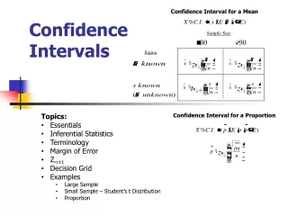
6.1 Confidence Intervals for the Mean (Large Samples). Statistics Spring Semester Mrs. Spitz. Objectives/Assignment. How to find a point estimate and a maximum error of estimate How to construct and interpret confidence intervals for the population mean

E N D
6.1 Confidence Intervals for the Mean (Large Samples) Statistics Spring Semester Mrs. Spitz
Objectives/Assignment • How to find a point estimate and a maximum error of estimate • How to construct and interpret confidence intervals for the population mean • How to determine the required minimum sample size when estimating • Assignment: pp. 259-261 #1-40 all
Estimating Population Parameters • In this chapter, you will learn an important technique of statistical inference—to use sample statistics to estimate the value of an unknown population parameter. In this particular section, you will learn how to use sample data to make an estimate of the population parameter when the sample size is at least 30 or the standard deviation is known. To make such an inference, begin by fnding a point estimate.
DEFINITION • A point estimate is a single value estimate for a population parameter. The most unbiased point estimate of the population mean is the sample mean .
Ex. 1: Finding a Point Estimate • Market researchers use the number of sentences per advertisement as a measure of readability for magazine advertisements. The following represents a random sample of the number of sentences found in 54 advertisements. Find a point estimate of the population mean . So, your point estimate for the mean length of all magazine advertisements is 12.4 sentences.
You try it: Finding a Point Estimate • Another random sample of the number of sentences found in 30 magazine advertisements is listed below. Use this sample to find another point estimate of the population mean . • Find the sample mean. • Estimate the mean sentence length of the population.
More about point estimates • In Example 1, the probability that the population mean is exactly 12.4 is virtually zero. So, instead of estimating to be exactly 12.4, you can increase your accuracy by estimating that it lies within an interval. This is called “making an interval estimate.”
More about interval estimates • Although you can assume that the point estimate in Example 1 is not equal to the actual population mean, it is probably close to it. To form an interval estimate, use the point estimate as the center of the interval, then add and subtract a margin of error. For instance, if the margin of error is 2.1, then an interval estimate would be given by 12.4 ± 2.1 or 10.3 < < 14.5. The point estimate and interval estimate are as follows. Before finding an interval estimate, you should first determine how confident you need to be that your interval contains the population mean .
Study Tip: • In this course, you will usually use 90%, 95%, and 99% levels of confidence. The following z-scores correspond to these levels of confidence.
DEFINITION • The level of confidence, c, is the probability that the interval estimate contains the population parameter.
Critical Values • You know from the Central Limit Theorem that when n ≥ 30, the sampling distribution of sample means is a normal distribution. The level of confidence, c, is the area under the standard normal curve between the critical values, -zc and zc.
Critical Values • You can see from the graph that c is the percent of area under the normal curve between -zc and zc. The area remaining is 1 – c, so the area in each tail is ½ (1 – c). For instance, if c = 90%, then 5% of the area lies to the left of -zc = -1.645 and 5% lies to the right of zc = 1.645
Error of Estimate • The distance between the point estimate and the actual parameter value is called the error of estimate. When estimating , the error of estimate is the distance • In most cases, of course, is unknown and varies from sample to sample. However, you an calculate a maximum value for the error if you know the level of confidence and the sampling distribution.
DEFINITION • Given a level of confidence, the maximum error of estimate (or error tolerance), E, is the greatest possible distance between the point estimate and the value of the parameter it is estimating. • When n ≥ 30, the sample standard deviation s can be used in place of .
Ex. 2: Finding the Maximum Error of Estimate • Use the data in Example 1 and a 95% confidence interval to find the maximum error of estimate for the number of sentences in a magazine advertisement.
Ex. 2: Finding the Maximum Error of Estimate--Solution • The z-score that corresponds to a 95% confidence interval is 1.96. This implies that 95% of the area under the curve falls within 1.96 standard deviations of the mean. You don’t know the populations standard deviation . But because n ≥ 30, you can use s in place of .
Ex. 2: Finding the Maximum Error of Estimate--Solution Using the values zc = 1.96, s ≈5.0, and n = 54. You are 95% confident that the maximum error of estimate is about 1.3 sentences per magazine advertisement.
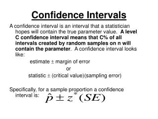
Confidence Intervals for the Population Mean • Using a point estimate and a maximum error of estimate, you can construct an interval estimate of a population parameter such as . This interval estimate is called a confidence interval.
Ex. 3: Constructing a Confidence Interval • Construct a 95% confidence interval for the mean number of sentences in a magazine advertisement. • Solution: In examples 1 and 2, you found that = 12.4 and E = 1.3. The confidence inteval is as follows:
Insight: • A larger sample size tends to give you a narrower confidence interval—for the same level of confidence.
Ex. 4: Constructing a Confidence Interval using Technology • Use a graphing calculator to construct a 99% confidence interval for the mean number of sentences in a magazine advertisement, using the sample in Example 1. • Solution: To use a calculator to solve the problem, enter the data and find that the sample standard deviation is s≈ 5.0. Then, use the confidence interval command to calculate the confidence interval (ZInterval for the TI-83 or TI-84). The display should look like the one on the next slide.
http://calculator.maconstate.edu/confidence_int_z/index.html#http://calculator.maconstate.edu/confidence_int_z/index.html# So, a 99% confidence interval for is (10.7, 14.2). With 99% confidence, you can say that the mean number of sentences is between 10.7 and 14.2.
More about intervals • In Ex. 4, and Try it Yourself 4, the same sample data was used to construct intervals with different levels of confidence. Notice that as the level of confidence increases, the width of the confidence interval also increases. In other words, using the same sample data, the greater the level of confidence, the wider the interval.
In Ex. 5, notice that if is known, then the sample size can be less than 30. • A college admissions director wishes to estimate the mean age of all students currently enrolled. In a random sample of 20 students, the mean age is found to be 22.9 years. From past studies, the standard deviation is known to be 1.5 years. Construct a 90% confidence interval of the population mean age.
In Ex. 5, notice that if is known, then the sample size can be less than 30. • The 90% confidence interval is as follows: So, with 90% confidence, you can say that the mean age of the students is between 22.35 and 23.45 years.
Interpreting the results • After constructing a confidence interval, it is important that you interpret the results correctly. Consider the 90% confidence interval constructed in ex. 5. Because already exists, it is either in the interval or not. It is not correct to say, “There is a 90% probability that the actual mean is in the interval (22.51, 23.29.” • The correct way to interpret your confidence interval is, “There is a 90% probability that the confidence interval you described contains .” This means also, of course, that there is a 10% probability that your confidence interval WILL NOT contain .
Sample Size • As the level of confidence increases, the confidence interval widens. As the confidence interval widens, the precision of the estimate decreases. One way to improve the precision of an estimate without decreasing the level of confidence is to increase the sample size. But how large a sample size is needed to guarantee a certain level of confidence for a given maximum error of estimate?
Ex. 6: Determining a Minimum Sample Size You want to estimate a mean number of sentences in a magazine advertisement. How many magazine advertisements must be included in the sample if you want to be 95% confident that the sample mean is within one sentence of the population mean?
Ex. 6: Determining a Minimum Sample Size Using c = 0.95, zc = 1.96, s ≈5.0 (from example 2), and E = 1, you can solve for the minimum sample size, n. When necessary, round up to obtain a whole number. So, you should include at least 97 magazine advertisements in your sample. (You already have 54, so you need 43 more.)