Download

1 / 73
730 likes | 887 Vues
Sighting-In on COLA. Vaš Majer Integral Systems, Inc AIAA Space Operations Workshop 15-16 April 2008 10/1/2014 12:06 AM. Introduction. Hello. Agenda. Parametric Analysis of Two COLA (Collision Avoidance) Statistics Probability of Collision, pC Commonly Used COLA Statistic

E N D
Sighting-In on COLA Vaš Majer Integral Systems, Inc AIAA Space Operations Workshop 15-16 April 2008 10/1/2014 12:06 AM
Introduction Hello
Agenda • Parametric Analysis of Two COLA (Collision Avoidance) Statistics • Probability of Collision, pC • Commonly Used COLA Statistic • Risk of Collision, rC • OASYS™ COLA Statistic • But First, a Discussion of GHRA...
GHRA Ground-Hog Risk Assessment
Background • Nicole Keeps a Garden • Ground-Hogs Like the Garden • She Tried • Sharing with Them • Reasoning with Them • Trapping Them
It’s Come to This: • .243 Varmint Rifle for Christmas • Quarter-Size Pattern at 100 m • After the Scope is Sighted-In • Sighting-In • Rifle Locked in Vise • Target Set @ 100 m • Scope Trained on Target at (0,0)
Scope Trained on Origin (0,0) Target @ 100 m Cross-Hair @ (0,0) 2 cm Dia Ref Ring, S Rifle Locked in Vise
Sighting-In Paradigm • Truth, Z=(Zx,Zy) • Barrel Bore-Sight Location on Target @ 100 m • Fixed but Unknown [Not a Random Variable] • Observations/Measurements, z=(zx,zy) • Bullet Hole Coordinates on Target @ 100 m • Subject to Dispersion • Estimator/Predictor of Truth, U=(Ux,Uy) • Scope Cross-Hair Coordinates on Target @ 100 m • Fixed and Known [Not a Random Variable] • U = (0,0) in Sighting-In Set-Up • Estimator Correction, u = (ux,uy) • Scope Cross-Hair Sighting-In Adjustment • To Be Determined
z,Z in Observation Space • z = Z + w, w = Gauss(0,W) • Z ~ barrel bore-sight coordinates • z ~ bullet hole coordinates • w ~ an instance of sample error • W ~ bullet dispersion covariance • Known or To Be Discovered • 0 ~ mean bullet dispersion • Z is Fixed, Unknown Bore-Sight Truth • z is Random Variable on Bore-Sight Space
u,U in Estimator Space • u = Z-U • U is Known [Cross-Hair] • Z is Fixed But Unknown [Bore-Sight] • u is Fixed And Also Unknown [Bias] • Z,U,u are Deterministic Values [Truth] • No Probabilities Are Involved • Can’t Hit Anything Either
The Connection z : u • Sample z: {zk, k=1:n} • Estimate un • Observation Model • zk = U + un + wk, k=1:n • wk ~ Gauss(0,W) • Making the Connection is a Model • u,U Domain of Model • z,Z Range of Model • Objective: Align Scope ~ Bore-Sight
The Confusion • un is Fixed, Deterministic, Computable • For a Given Trial of n Samples, {zk, k=1:n} • un is a Random Variable • On the Space of All Trials of n Samples,{zk,j, k=1:n, j=1:∞} • un Wears Two Hats
3 Rounds Fired Rounds ~ Red Dots High and Right Need More Observations Cheap Rounds are $2 Each This Info Cost $6
Triangulation “Two Rounds are Not Enough; Four are too Many” Barycenter of Triangle Scope Adjusters 1 click = 1 cm Could Sight-In Scope Now...But We Won’t
100 Rounds Fired Calibrated Eyeball Suggests Bore Location ~ (1 cm, 3 cm) This Single Trial of100 Rounds Cost $200 This Information Cost $200
100 Sample Mean & Covariance u100 ~ + W100 ~ O R100 ~ O
Sample Mean & Covariance • Mean of n Samples (n=100) • + un = (1/n) Σk=1:n zk • Covariance of n Samples (n=100) • O Wn = [1/(n-1)] Σk=1:n (zk-un)(zk-un)T • Wn = [ anan cnanbncnbnan bnbn] • an, bn > 0; -1 ≤ cn ≤ 1
Sample Space Properties • un→ u as n → ∞ • un ~ Finite Sample Mean • u ~ Infinite Sample Mean aka Truth • Wn→ W as n → ∞ • Wn ~ Observation Residual Covariance • W ~ Dispersion of Rounds in Z-Space • (u,W)Define a Metric on the Z-Space • J(z; u,W) = (z-u)T W-1 (z-u) = (-)T(-) • = W-½z = W-½u (Silly Putty Transform) • Red Ellipse is Unit Sphere in (un,Wn) Silly Putty Metric • Scale in cm of 1 Unit of (un,Wn) Metric • Depends on Direction of (z-un)
Parameter Space Properties • + un = argminvΣk=1:n J(zk; v,W) MinVariance/MaxLikelihood • 0 R-1n = Σk=1:n W-1 Fisher Information • Rn ~ Dispersion of Estimators Over Many Trials of n Samples • Covariance of un when Wearing its Trial Hat • Rn = (1/n) W • Rn→ 0 as n → ∞ • (u,R)Define a Metric on the U-Space • J(v; u,R) = (v-u)T R-1 (v-u) = (-)T(-) • = R-½z = R-½u • Green Ellipse is Unit Sphere in (un,Rn) Silly Putty Metric • Scale in cm of 1 Unit of (un,Rn) Metric • Depends on Direction of (v-un) • And → 0 as n → ∞ ! • (un,Rn) Metric is Smaller Scale than (un,Wn) Metric • Reflects the Information Packed into R-1n from n Samples
Wait A Minute... • Are not u,U and z,Z the Same Spaces? • Yes, They Are All Fruit • Vectors in the Target Plane • No, They Are Not the Same • Apples ~ Model Domain • u,U Corrected/Prior Scope Cross-Hair Locations • Oranges ~ Model Range • z,Z Observed/True Bore-Sight Locations
200 Sample Mean & Covariance u200 ~ + W200 ~ O R200 ~ O This is a Virtual Trial only to Illustrate n=200 Another $400 for Ammo is Out of the Question
More Information (n=200) • un,Wn Adjust Slightly • Centroid and Dispersion of Rounds are Revealed Slightly Better w/ 200 Rounds • Rn is Cut in Half (100/200) • Reflects the Doubling of Information • R½n Metric on u,U-Space is Cut By 1/√2 • u200 is NOT √2 Times More Accurate than u100 • Nicole...I Didn’t Fire 200 More Rounds
Adjust Scope to 100 Sample Mean I Can Afford only 1 Trial of n=100 Samples u100 is Best Estimator of Bore-Sight LocationGiven n=100 Samples Treat u100 as if it WERE the True Bore-Sight Location Adjust Cross-Hair on u100 Rifle Still Clamped in Vise
But What if I... • Had 99 More Boxes of 100 Rounds? • Ran 99 More Trials of 100 Samples? • un,j, Wn,j, Rn,j • n=100 for each Trial • Trials j=1:m, m=100 • 10K Rounds
Means for 100 TrialsEach Trial having 100 Samples + Trial Means, un,j * Mean over Trials, un* O Sample Covariance over Trials, P O Estimator Covariance over Trials, R Scope is Trained on u100 for Trial 1 Nicole, I Didn’t Spend $20K on Ammo
Zoom-In On Mean of Means + un,j for n=100 * un* O Sample Covariance, P O Estimator Covariance, R Scope is Still Trained on un,1
What’s the Truth? • Truth is Un-Obtanium Given... • Finitely Many Samples (e.g., n=100) • No un,j is Truth • It’s Simply A Different Trial of n=100 Samples • Even un* = Mean(un,j) = Mean of Means is Not Truth • But un* Converges to Truth as n → ∞ • Just as un,j Converges to Truth as n → ∞ for any fixed j • In Real Life We Get Only 1 Trial • Make n as Large as Affordable (Number of Rounds) • Make W as Small as Affordable (Quality of Rounds) • We Treat un,1 As if It Were Truth ( Working Hypothesis) • Fixed and Known, Deterministic not Probabilistic • The Best Estimator/Predictor We Have or Can Afford • The Practical Truth on Which We Base Operational Decisions
For All Practical Purposes... • Drop the n... • u := un • Adjust the Scope... • U := U+u = u • Bore-Sight := Scope Cross-Hairs on... • Z = U = u • Fire 1 Round... • z = u + w, w ~ (0,W) • If z is not within Scope Reference Ring, S... • Buy $3 Rounds with Smaller Dispersion, W
Role of Estimator Covariance, R • R is a Cruel Hoax • Estimator Algorithm Yields (u,R) • R is Centered on Z, Which is Unknown • u-Z is Unknown Bias • R is Notoriously Optimistic • R → 0 ~ 1/n → 0, n = Sample Size • No Comparable Convergence for Rate u → Z with n • Having No Alternative... • We Define Z := u (Working Hypothesis) • Center R on u • Consider v ~ Gauss(u,R) in U-Space • v are Trial Estimators • Every v in u,U-Space is a Possible Estimator • u is MinVariance/Max Likelihood Estimator • The Best Estimator [We Can Afford; Given the Observations]
We Add to Confusion... • By Suppressing/Discarding z,Z • Once u,R Have Been Computed • And then Switching Notation from • v ~ Gauss(u,R), U = Truth • v is Trial Variable in Estimator Space • To • z ~ Gauss(u,R), Z = Truth • Now z is Trial Variable in Estimator Space
Uses of Estimator Covariance, R • R ~ Dispersion of Estimators, u • With Respect to Truth, Z, over Many Trials • R ~ Uncertainty Metric on u,U-Space • R is NOT the Accuracy, |u-Z|, of u • In Our Example: |u – Z| ~ 2 R-Units • R Should be Constant across Trials • Use R to QA Estimation Process • Variation from Trial to Trial Signals that Trials are Not Comparable
GHRA Summary v ~ Gauss(u,R)
v ~ Gauss(u,R), v in U-Space • u is Fixed U-Vector • R is Fixed Covariance • v is Trial or Dummy Variable • J(v; u,R) is Squared Length of v-u w/r R-metric • p = ∫Q dp(v; u,R) is Probability-Weighed Measure of Set Q w/r R-metric • dp(v; u,R) = [1/(2π)|R|1/2] exp[-J(v; u,R)/2] dv • v is Variable of Integration over Q • 0 ≤ p < 1 for Bounded Sets Q • p = 1 for Q = Entire U-Space • p is NOT • Probability that Truth, Z, Lies in Q • p is • Probability that v Selected Randomly from Gauss(u,R) lies in Q • A Measure of Set Q with Rapidly Decreasing Weight Centered @ u
COLA Collision Risk Assessment
Given • t → u(t) • 3D Separation Vector Ephemeris • Vehicle Y with Respect to Vehicle X • u=0 @ Vehicle X Center of Mass • t → R(t) • 3D Joint Uncertainty Covariance Ephemeris
Common Practices • Reduce Dynamic to Static • Restrict Attention to Time[s] of Closest Approach • Reduce 3D to 2D • Remove Dimension Along Velocity Vector
The Scenario Looks Familiar u Separation Estimate R Covariance of Estimator d Radius of Hard Body Stay-Out Sphere, S z = (x,y) Any Trial Vector TRUTH, z=Z, is, As Always, Nowhere to be Seen, FixedBut Unknown
The Definition • Collision • TRUTH, Z, is Inside Stay-Out Sphere S
The Objective • Quantify Risk of Collision • For Given Estimator, u • In View of Uncertainty, R • In View of Stay-Out Sphere, S • With a Single Number, r
Attributes of Risk Statistic, r • 0 < r ≤ 1 • r = 0 Lowest Possible Risk • r = 1 Highest Possible Risk • r is Conservative • r is Robust
Conservative • Because Estimator, u... • Is Biased • Bias u-Z is Unknown • And Because Estimator Covariance, R... • Should be Centered on Truth, Z, which is Unknown • Is Notoriously Optimistic [Small] • Under-States Variance/Uncertainty • We Want Risk Statistic, r, Such That... • r is Upper Bound on Risk • r Threshold Levels Have MeaningIndependent of Scenario Geometry • r > 0; Risk Never Sleeps • r = 1 OK; Extreme Risk Deserves Notice
Robust • r Conforms to Intuitive Notion of Risk • r increases as |u| decreases • r increases as |R| increases • r increases as d increases • r is Sensible for Limiting Scenarios • u in S implies r = 1 • u near S implies r ~ 1 • r makes sense even for d=0
COLA Statistic Definitions Two Statistics
Probability of Collision, pC Commonly Used COLA Statistic
Probability of Collision, pC pC = ∫S dp(z; u,R) dp(z) = [1/(2π)n/2|R|1/2] exp[-J(z; u,R)/2] dz • pC = Integral over S of Gauss(u,R) Density • dp(z) = Gauss(u,R) Density • S = Sphere of Radius d Centered @ Origin • Here n = 3, Dimension of 3-Space
Probability of Collision Heuristic* • dp(z) = Probability Density of True Separation, Z, w/r to u • pC = Probability that True Separation, Z, is Inside Sphere S *R.P. Patera, General Method for Calculating Satellite Collision Probability, AIAA J Guidance, Control and Dynamics, Vol 24, No 4, July-August 2001, pp 716-722.
Risk of Collision, rC OASYS™ COLA Statistic
Risk of Collision, rC • if (0 ≤ |u| ≤ d) rC = 1; • else v = d (u/|u|); V = {z | J(z; v,R) < J(u; v,R)} q = ∫V dp(z; v,R) rC = 1 – q;
Risk of Collision Heuristic • Make the NULL Hypothesis: • u is a Trial Estimator of Z=v, where • v = d (u/|u|); d = radius of S; and • Trial Estimators are z ~ Gauss(v,R) • v is the Point in S which is Closest to Estimator u • V is the (v,R) Metric Sphere of Radius |R-1/2(u-v)| Centered at v • Estimator u is on the Boundary of V • q is • the Probability Measure of the (v,R)-Sphere, V • the Probability that a Random Trial Estimator of Z=v Lies in V • rC = 1-q is • the Probability Measure of the Complement of V • an Upper Bound on the Probability that the NULL Hypothesis is TRUE
Parametric Comparison pC and rC Over a Family of Scenarios