Time Response, Stability, and Steady State Error

1. Time Response, Stability, and Steady State Error CEN455: Dr. Nassim Ammour

2. 1 Time Response • The mathematical representation of a system (Transfer function or State space) is used to analyze its transient and steady-state responses to see if these characteristics yield the desired behavior. • Performance of controlled systems can be tested and compared by their responses to certain test signals (Step functions, impulse functions, ramp functions, sinusoidal functions, etc.). • A response of a dynamic system can be analyzed in two parts: • Steady-state response: The behavior of the output as • Transient response: The behavior of the output as it goes from an initial state to a final state. • This chapter is devoted to the analysis of system transient response. CEN455: Dr. Nassim Ammour

3. Time Response Poles, Zeros, and System Response • The output response of a system is the sum of two responses: • 1. the forced response (steady-state response or particular solution), • 2. the natural response (the homogeneous solution). Output response = forced response (e.g. constant) + natural response (e.g. exponential) roots of the denominator (characteristic polynomial) of the transfer function • Poles of a Transfer Function (TF): The values of sthat cause • Zeros of a TF: the values of sthat cause TF = 0. roots of the numerator of the transfer function Example: Poles and Zeros of a First-Order System System Output (unit step response) where and System showing input and output Inverse Laplace transform: System Output in time domain (time response) pole-zero plot of the system CEN455: Dr. Nassim Ammour

4. Example: Poles and Zeros of First Order System Input function generates Input poles Forced response ( pole at the origin generated a step function at the output) generates System poles Natural response Transfer function (A pole on the real axis generates an exponential response of the form that will decay to zero). System poles And zeros generates Amplitudesfor both the forced and natural responses Evolution of a system response. CEN455: Dr. Nassim Ammour

5. Evaluating Response using Poles Problem: Given the following system, write the output, c(t), in general terms. Specify the forced and natural parts of the solution. Solution: Forced response Natural response Taking inverse Laplace transform, • Each system pole generates an exponential as part of the natural response. • The input's pole generates the forced response. Poles of the system produce the Natural response that Will decay to zero CEN455: Dr. Nassim Ammour

6. First-Order System: Time Constant • A first-order system without zero: • If the input is a unit step: then the Laplace • transform of the step response is : the input pole at the origin generated the forced response • Taking the inverse transform The system pole at –a generated the natural response • Significance of parameter a (system pole) (only parameter needed to describe the transient response), When Hence, CEN455: Dr. Nassim Ammour

7. Some Terminology (three transient response performance specifications). 1. Time constant : Time it takes for the step response to rise to 63% of its final value. • we can call the parameter (system pole) the exponential frequency (The reciprocal of the time constant) • is related to the speed at which the system responds to a step input. 2. Rise Time : Rise time is defined as the time for the response to go from 0.1 to 0.9 of its final value. found by solving for the difference in time at c() = 0.9 and c() = 0.1 Rise time: 3. Settling time : The time for the response to reach, and stay within, 2% of its final value. Lettingand solving for time, , we find the settling time to be CEN455: Dr. Nassim Ammour

8. First-Order Transfer Function via Testing • With a step input, we can measure the time constant and the steady-state value, from which the transfer function can be calculated. • A simple first order system has : and step response is: In the time domain (ILT): • From the response, we identify Kand ato obtain the transfer function. To find a: To find K: From , the forced response reaches a steady-state value of Transfer function, and CEN455: Dr. Nassim Ammour

9. Second-Order System1 • Parameters of First-order system determine the speed of the system. • Parameters of Second-order system determine the form (shape) of the system. System poles Consider the general system, • For un-damped(without damping) system, , and the poles are on at , Natural Frequency Hence un-damped system • For an under-damped system, poles have real part (exponential decay ), Exponential decay frequency General case of second order system D Natural frequency : (Natural Frequency ) the frequency of oscillation of the system without damping. (D) dimensionless measure describing how oscillations in a system decay. exponential decay , real part of the pole Poles Canonical form (two finite poles and no zeros) CEN455: Dr. Nassim Ammour

10. Second-Order System2 The sign of the discriminant of the denominator polynomial depends on the damping ratio , three cases. System poles Case1: Overdamped system: () Two real poles the general case (two finite poles and no zeros) Overdamped system CEN455: Dr. Nassim Ammour

11. Second-Order System Case 2: Under-damped Response () : (Two complex poles that come from the system). Poles from the system: exponential decay frequency of the sinusoidal oscillation. From, Second-order step response components generated by complex poles Where, CEN455: Dr. Nassim Ammour

12. Second-Order System Case 3: Un-damped Response (: pole at the origin that comes from the input and two imaginary poles that come from the system. Case 4:Critically Damped Response ( : pole at the origin that comes from the input and two multiple real poles that come from the system. 3 There is no exponential term, so no decay. There is no sinusoidal term, so no oscillation. CEN455: Dr. Nassim Ammour

13. Second-Order System Over-damped responses Two Two real poles at All Together Two Under-damped responses Two complex poles at Un-damped responses Two Two imaginary poles at Critically damped responses Two Two real poles at Step responses for second-order system damping cases CEN455: Dr. Nassim Ammour

14. Second-Order System As a Function of Damping Ratio • Relationship between the quantities and the pole location. Solving for the poles of the transfer function Example For the system find the value of and report the kind of response expected. We have and System is over-damped. CEN455: Dr. Nassim Ammour Second-order response as a function of damping ratio

15. Underdamped Second-Order Systems • The nature of the response obtained is related to the value of the damping ratio (over-damped, critically damped, underdamped, and un-damped responses.). • Step response for the general second-order system, Expanding by partial fractions, (< 1 the underdamped case ) The lower the value of ζ, the more oscillatory the response is. inverse Laplace transform Where, CEN455: Dr. Nassim Ammour Second-order underdamped responses for damping ratio values

16. Underdamped Second-Order Systems Specifications • Other parameters associated with the underdamped response are rise time, peak time, percent overshoot, and settling time. The time required for the waveform to go from 0.1 of the final value to 0.9 of the final value. Rise time Second-order underdamped response specifications The time required to reach the first, or maximum, peak. Peak time The amount that the waveform overshoots the steady-state, or final, value at the peak time, expressed as a percentage of the steady-state value. percent overshoot and The time required for the transient's damped oscillations to reach and stay within ±2% of the steady-state value. settling time Derivation: self study. CEN455: Dr. Nassim Ammour

17. Under-damped Second-Order Systems Specifications (continued) from the Pythagorean theorem Damped frequency of oscillation damped frequency of oscillation, Damping Ratio Natural frequency inversely proportional to the imaginary part of the pole. inversely proportional to the real part of the pole. exponential damping frequency. CEN455: Dr. Nassim Ammour

18. Under-damped Second-Order Systems Step Response as Pole moves poles move in a vertical direction (with constant real part ) • frequency increases • envelope remains the same (constant real part ) • settling time is virtually the same • overshoot increases, the rise time decreases poles move in a horizontal direction (with constant imaginary part ) • As the poles move to the left, response damps out more rapidly. • peak time is the same for all waveforms (constant imaginary part ) poles move in along a constant radial line direction • The percent overshoot remains the same. • The farther the poles are from the origin, the more rapid the response. CEN455: Dr. Nassim Ammour

19. Finding TP, %OS, and TS From Pole Location Problem: Given the pole plot find , , , %OS, and . Solution: Damping ration, Natural frequency, Peak time, Percent overshoot, The approximate settling time, CEN455: Dr. Nassim Ammour

20. System Response with Additional Poles • If a system has more than two poles or has zeros, we cannot use the formulas to calculate the performance specifications that we derived. • We need to approximate that system to a second-order system that has just two dominant complex poles. And the real pole at Assuming two complex poles at Time domain step response, CEN455: Dr. Nassim Ammour

21. Comparing Responses of Three-Pole Systems if the real pole is five times farther to the left than the dominant poles system is represented by its dominant second-order pair of poles. CEN455: Dr. Nassim Ammour

22. Evaluating Pole-Zero Cancellation Effect of a zero on the system: A system with a zero consists of the derivative of the original response and the scaled version of the original response. If the zero is very large, the Laplace transform of the response is approximately the scaled version of the original response. As the zerobecomes smaller, the derivative term contributes more to the response and has a greater effect. derivative response scaled response pole-zero cancellation Problem: For any function for which pole-zero cancellation is valid, find the approximate response. Effect of adding a zero to a two-pole system Solution: The partial-fraction expansion of is That residue (1) is not negligible. So a 2nd-order step response approximation cannot be made for . The partial-fraction expansion of is That residue (0.033) is negligible, so cancel zero and that pole. Hence, the approximate response, CEN455: Dr. Nassim Ammour

23. 2. Stability Stability is the most important system specification. the total response of a system Stable system: If natural response approaches zero as time approaches infinity (LTI System). Marginally stable system: If natural response neither decays nor grows but remains constant or oscillates as time approaches infinity. BIBO (Bounded Input, Bounded Output) yields stable system. Stable systems have closed-loop transfer functions with poles only in the left-half plane. CEN455: Dr. Nassim Ammour

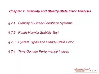
24. Routh-Hurwitz Criterion This method Provides stability information with solving for system poles. How many poles are in left / right plane or in jw axis, not where Routh Table Generation: Completed Routh table Denominator: CEN455: Dr. Nassim Ammour

25. Routh-Hurwitz Criterion: Example Make the Routh table for the system shown in Figure PROBLEM: The first step is to find the equivalent closed-loop system SOLUTION: Interpreting the Basic Routh Table How many signchanges in the first column  the number of poles in the right-half plane Two such poles : unstable system. Any row can be multiplied by a positive number. the row was multiplied by 1/10 the number of roots of the polynomial that are in the right half-plane is equal to the number of sign changes in the first column. the first column CEN455: Dr. Nassim Ammour

26. Routh-Hurwitz Criterion: Special Cases 1. Zero Only in the First Column If the first element of a row is zero, division by zero in the next row Example: CEN455: Dr. Nassim Ammour

27. Routh-Hurwitz Criterion: Special Cases Zero Only in the First Column: reverse coefficients The polynomial that has the reciprocal roots of the original, is another method that can be used when a zero appears only in the first column of a row. reciprocal roots (s is replaced by l/d), Since there are two sign changes, the system is unstable and has two right-half-plane poles Example: Reverse coefficients: CEN455: Dr. Nassim Ammour

28. Routh-Hurwitz Criterion: Special Cases 2. Entire Row is Zero An entire row consists of zeros because there is an even polynomialthat is a factor of the original polynomial (only even powers of s and have roots that are symmetrical about the origin.) Example: Derivative of the polynomial of the row above the zeros row the row was multiplied by 1/7 entire row consists of zeros Stable system. CEN455: Dr. Nassim Ammour

29. Pole Distribution via Routh Table with Row of Zeros PROBLEM: Tell how many poles are in the right half-plane, in the left half-plane, and on the jw-axis. :Even polynomial Taking the derivative the row was multiplied by 1/10 Two sign changes the row was multiplied by 1/20 entire row consists of zeros the row was multiplied by 1/2 interpretation No sign change CEN455: Dr. Nassim Ammour

30. Stability Design via Routh-Hurwitz Changes in the gain K of a feedback control system change the closed-loop pole locations (can move poles from region to another region on the S-plane). Find the range of gain, K, for the system that will cause the system to be stable, unstable, and marginally stable. Assume K > 0. PROBLEM: Variable gain K 1. If K < 1386, then stable system. 2. If K > 1386, then two sign changes; two right-half plane poles and one left-half plane pole. Unstable system. 3. If K = 1386, an entire row of zeros  j poles. replacing K=1386 No sign change can be positive, zero, or negative Row of zeros 2 poles in j axis and one left-half plane pole no sign changes above the even polynomial the system is marginally stable CEN455: Dr. Nassim Ammour

31. Factoring via Routh-Hurwitz The Routh-Hurwitz criterion is often used in limited applications to factor polynomials containing even factors. PROBLEM: Factor the polynomial (1) (2) • Dividing polynomial (1) by (2) yields: CEN455: Dr. Nassim Ammour

32. Stability in State Space • The values of the system's poles are equal to the eigenvalues of the system matrix, A. PROBLEM: find out how many poles are in the left half-plane, in the right half-plane, and on the jw-axis. SOLUTION: Using this polynomial, form the Routh table one sign change: One right-half-plane pole and two left-half-plane poles. Unstable system. CEN455: Dr. Nassim Ammour

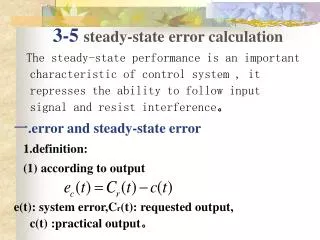
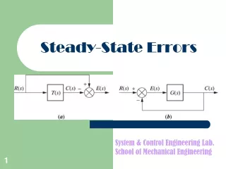
33. 3. Steady-State Errors Steady-State Error: The difference between the input and the output for a prescribed test input (step / ramp / parabola) as t Test waveforms for evaluating steady-state errors of position control systems step input ramp input Steady-state error CEN455: Dr. Nassim Ammour

34. Evaluating Steady-State Errors1 Error output input Problem: Find the steady-state error for the following system with Closed-loop control system error and input is step response. Solution: Step input Applying final value theorem We have the error T(s) is stable, hence E(s) is stable. Applying final value theorem, CEN455: Dr. Nassim Ammour

35. Evaluating Steady-State Errors2 Ramp input: tu(t) For zero steady-state error, [Final-value theorem] Parabolic input: (1/2)t2u(t) Step input: u(t) For zero steady-state error, For zero steady-state error, CEN455: Dr. Nassim Ammour

36. Evaluating Steady-State Errors example1 u(t): unity step Problem: Find steady-state errors for inputs 5u(t), 5tu(t), and 5t2u(t) to the above system. Solution: Let, the system is stable. CEN455: Dr. Nassim Ammour

37. Evaluating Steady-State Errors-example2 One integration, s1 No integration will make it constant, one integration makes it zero. No integration will make it infinity. one integration makes it constant. Two integrations will make it constant and 3 or more will make it zero. CEN455: Dr. Nassim Ammour

38. Static Error Constants The steady-state error performance specifications are called staticerror constants. steady-state error. PROBLEM: evaluate the static error constants and find the expected error for the standard step, ramp, and parabolic inputs. step input, u(t) ramp input, t u(t) Position constant, Kp: Velocity constant, Kv: Acceleration constant, Ka: CEN455: Dr. Nassim Ammour

39. System Type Type 0: if n = 0; (no integration) Type 1: if n = 1; (one integration) Type 2: if n = 2; (two integrations) Problem: Find the value of K so that there is 10% error in the steady state. Input should be ramp, because only ramp yields a finite error in Type 1 system. Solution: Type 1. CEN455: Dr. Nassim Ammour

40. System Type Relationships between input, system type, static error constants, and steady-state errors CEN455: Dr. Ghulam Muhammad

41. Steady-State Error for Disturbances Feedback control systems are used to compensate for disturbances or unwanted inputs that enter a system. disturbance Problem: Find the steady-state error component due to a step disturbance Solution: steady-state error due to R(s), steady-state error due to disturbance D(s), steady-state error due to step disturbance D(s)=1/s, CEN455: Dr. Nassim Ammour

42. Steady-State Error for Nonunity Feedback System Form a unity feedback system by adding and subtracting unity feedback paths (input and output units must be same.). PROBLEM: Find the system type, error constant, and the steady-state error for a unit step input. Type 0 (as no integration). For step input, static error constant is Kp. Negative value means the output step is larger than the input step. CEN455: Dr. Nassim Ammour