Download
1 / 29
390 likes | 926 Vues
Dosing Regimen Design. Multiple Dosing: Intermittent or multiple dose regimen. 100 mg q. t 1/2 via i.v. bolus. 200. 150. Amount in Body [mg]. 100. 50. Time [t 1/2 ]: 1 2 3 4 5 6. Principle: 1 dose lost per .

E N D
Dosing Regimen Design Multiple Dosing: Intermittent or multiple dose regimen
100 mg q. t1/2 via i.v. bolus 200 150 Amount in Body [mg] 100 50 Time [t1/2]: 1 2 3 4 5 6
Principle: 1 dose lost per At steady state, Rate In = Rate Out F•Dose = Ass,max - Ass,min Ass,min = Ass,maxe-KE F•Dose = Ass,max (1 - e-KE) Ass,max = F•Dose /(1 - e-KE) Ass,min = Ass,max - F•Dose
AN,max & AN,min N = 1 2 3 4 5 6 7 Not AN,min = AN,max - F•Dose Why?
Average amount of drug in the body at steady state At steady state, Rate In = Rate Out FDose/ = KE Ass,av 1/KE = t1/2/ln 2 = 1.44 t1/2
AUC Equal Areas
Css,av Concept applies to all routes of administration and it is independent of absorption rate.
Dosing rate from AUC0- Given AUC after a single dose, D, the maintenance dose, DM , is: Where D produced the AUC0-, Css,av is the desired steady-state plasma concentration, and is the desired dosing interval.
Example: 50 mg p.o. dose 2 3 2.4 1.8 Cp mg/L 1 2 4 8 Time [h] AUC = 1+2.5+5.4+8.4+6 = 23.3 mg•h/L
Example, continued Calculate a dosing regimen for this drug that would provide an average steady-state plasma concentration of 15 mg/L. DM = 193 mg Dosing regimen: 200 mg q. 6 h.
Example, continued - 2 There is a problem with this approach ?? Peak and trough concentrations are unknown. Css,max Css,min
Another example - digitoxin t1/2 = 6 days; usual DR is 0.1 mg/day Assuming rapid and complete absorption of digitoxin, Ass,av = 1.44 F Dose t1/2/ = (1.44)(1)(0.1mg/d)(6d)/(1d) = 0.864 mg What would be the average steady-state body level? Maximum and minimum plateau values? Ass,max = 0.1/(1-e-(0.116)(1)) = 0.909 mg Is there accumulation of digitoxin? Ass,min = 0.909 – 0.1 = 0.809 mg How long to reach steady state?
KE AI KE FI Rate of Accumulation, AI, FI The rate of accumulation depends on the half-life of the drug: 3.3 x t1/2 gives 90% of the steady-state level. Accumulation Index (AI): Ass,max/F DM = (1 – e-KE)-1 Fluctuation Index (FI): Ass,max/Ass,min = e+KE When = t1/2 AI = FI = 2
ka v CL Absorption Rate influence on Rate of Accumulation KE = 0.1
When ka >> KE, control is by drug t1/2: When ka << KE, control is by absorption t1/2:
Loading Dose (LD) = Ass,max F Whether a LD is needed depends upon: • Accumulation Index • Therapeutic Index • Drug t1/2 • Patient Need
Cp Time Dosing Regimen Design OBJECTIVE: Maintain Cp within the therapeutic window.
Cu Cp Cl max Time Dosing Regimen Design APPROACH: Calculate max and DM,max.
Cp Time DM,max and Dosing Rate From the principle that one dose is lost over a dosing interval at steady state: DM,max = (V/F)(Cu - Cl) The Dosing Rate (DR) is DM,max max
KEV = CL (Cu - Cl)/ln(Cu/Cl) = Css,av = logarithmic average of Cu and Cl. The log average is the concentration at the midpoint of the dosing interval; it’s less than the arithmetic average. DR = (CL/F)Css,av
Average Concentration Approach • Choose the average to maintain: Css,av = (Cu - Cl)/ln (Cu/Cl) • Choose : max ;usually 4, 6, 8, 12, 24 h • Calculate DR: DR = (CL/F)Css,av • Calculate DM: DM = DR•
Example Css,av = (10 – 3)/ln (10/3) = 5.8 mg/L max = (1.44)(4.85)[ln (10/3)] = 8.41 h Choose < max: 8 h DR = (5 L/h)(5.8 mg/L)/(0.8) = 36.25 mg/h DM = (36.25 mg/h)(8 h) = 290 mg 300 mg Dosing Regimen: 300 mg q 8 h
Peak Concentration Approach • Choose the peak concentration to maintain. • Choose : max ;usually 4, 6, 8, 12, 24 h • Calculate DM: DM = (V•Cpeak/F)(1 - e-KE) from:
Example Cpeak = 8 mg/L max = (1.44)(4.85)[ln (10/3)] = 8.41 h Choose < max: 6 h set to 6 h so that Css,min > Cl DM = [(35 L)(8 mg/L)/0.8](1 – e-(0.143)(6)) = 202 mg Dosing Regimen: 200 mg q 6 h
Check Css,max = [(0.8)(200)/35]/(1 – e-(0.143)(6)) = 7.93 mg/l Css,min = 7.93 - (0.8)(200)/35 = 3.4 mg/L
Rationale for controlled release dosage forms • Compliance vs. fluctuation: when the dosing interval is less than 8 h, compliance drops. • For short half-life drugs, either must be small (2, 3, 4, 6 h), or the fluctuation must be quite large, when conventional dosage forms are used. • Use of controlled release permits long while maintaining low fluctuation. • Not generally of value for drugs with long half lives (> 12 h). Due to extra expense, they should not be recommended.
Assessment of PK parameters CL: CL/F = (DM/)/Css,av and Css,av = AUCss,/ Relative F: CLR: CLR = (Ae,ss/ x Css,av) where Ae,ss is the amount of drug excreted in the urine over one .