Download
1 / 20
340 likes | 711 Vues
Oceanic Eddies. Byron Conley Work done at COAPS with: Dr. Brian Arbic Dr. Patrick Timko. Outline. I will address our goal: to use eddy tracks to explain persistent signals Clarify relevant concepts Introduce the previous work that has led to our project Describe our work

E N D
Oceanic Eddies Byron Conley Work done at COAPS with: Dr. Brian Arbic Dr. Patrick Timko
Outline • I will address our goal: to use eddy tracks to explain persistent signals • Clarify relevant concepts • Introduce the previous work that has led to our project • Describe our work • And, time–permitting: • Discuss the challenges, benefits, and related developments in our study of oceanic eddies
Goal Want to know if tracks of eddies, initially assumed isotropic, found in Chelton et al. (2007) can explain anisotropic signals seen described in Scott et al. (2008).
Clarifications • What is an eddy? • General Definition: rotational movement of fluid that occurs when a flow passes over/around an obstruction, between oppositely flowing currents, or along edges of permanent currents • Vortices • Contain most of the ocean’s kinetic energy • Inverse energy cascade of two-dimensional flows: nonlinear advection (loosely: transfer) shifts kinetic energy from small to large scales, resulting in persistent structures (our eddies) • Eddies generally contain much higher kinetic energy than the mean kinetic energy of the worlds ocean Convergence of Oyashio and Kuroshio currents, off Hokkaido, Japan
More on Eddies • Ocean’s dynamic equivalent of synoptic (large-scale) weather systems • Organization of turbulent fluid motion • “Stirring” mechanism through turbulent diffusion • Transfers heat, momentum, mass, chemical constituents of ocean: process known as “advection” • Anisotropy: quantification of preferred direction in flows • u=zonal (E-W) velocity, v=meridional (N-S) velocity, <> denotes time-average • For our purposes, M=<u2-v2>/<u2+v2> gives us an idea of how well structured, isotropic, or elongated, anisotropic, the eddies are. • M=0 indicates isotropy, ie. <u2>=<v2>; |M|≤1 • Idealized models of ocean eddies usually see M > 0 (Arbic et al. 2004 and references therein)
Geostrophic Balance • Geostrophic balance results from a balance between the pressure gradient and the Coriolis Effect • We use geostrophic approximation to determine the velocities that we have interest in for this project. (Useful poleward of ±5° Lat.) • How we get our zonal (u) and meridional (v) velocities These equations are derivations of the Navier-Stokes equations. “f” or Coriolis Parameter In these: Z = geopotential height, ie. our SSH (Sea Surface Height) measurements Approximation fails within a few degrees of the Equator The Coriolis Effect
Scott et al. • What does it tell us? • Research done on the zonal vs. meridional velocity variance from satellite observations and ocean models • Found that, in general, <u2>≠<v2>, therefore, eddies are generally anisotropic • Eddies can leave persistent signals over large timescales, counterintuitive to the chaotic nature of turbulent fluid motion • Typically have a general westward propagation • Persistent small-scale patches arise if they [eddies] follow preferred paths, perhaps due to bottom topography
Chelton et al. • Eddy tracking experiment • Uses data smoothed and filtered from original AVISO satellite data to accentuate the relevent eddy data, based on current eddy characterizations • Removes data for ssh anomalies with lifetimes < 21 days, with amplitudes < 5 cm • Typical eddy amplitudes ~5-25 cm • Typical eddy diameters ~100-200 km
Process • Form data matrix from provided eddy data • Write a program to read in the data from the two files to build our data matrix • Sort the info into files for each date, containing cyclonic and anticyclonic eddy data • Construct SSH fields using effective and e-folding eddy radii. • Determine optimum radius size, type, and decay factor. • Use visual and mathematical (% Variance Captured—more later) methods for these purposes. • From reconstructed SSH fields, determine u and v for all available data • Differentiate the SSH to get u and v • Repeat process for AVISO satellite data • Using u and v, calculate M-fields (remember M=<u2-v2>/<u2+v2>) for desired time periods. • Compare our reconstruction-based M-fields to AVISO-based M-fields • Hopefully, we will get comparable results • If these results are adequately similar, then we can answer the following questions and satisfy our goal: • Why does an isotropic eddy field still leave an anisotropic M-field? • Why is there temporal persistence?
SSH AVISO vs. Reconstruction • At first glance, it might seem that we are missing much of the SSH anomaly data • Smoothing and filtering techniques performed by Chelton et al. (our source of data) removed much of the unwanted data • Filtering/smoothing brings out much of the useful eddy data, while discarding much of the “noise’ • Visibly, the patterns are still fairly apparent • When performing our mathematical comparison, percent variance captured, we achieved expected results (~15-30% for the most effective reconstruction methods)
M-fields • Here is an example of an M-field construction • Image constructed by Scott et al. for 13 year time average (Oct. 11, 1992 – Jan. 21, 2006) • Our images (we hope) will look very similar
How persistent paths can leave signatures in the M field • As eddies propagate, their tracks leave trails visible in the M-fields • If we contour M>0 and M<0 as different colors, we can see these tracks • If another eddy takes a similar track, time averaging shows the preferred track • As stated before, can eddies which are individually isotropic still leave anisotropic signatures locally as in Scott et al. (2008)? • Can we explain the temporal persistence of these anisotropic signatures by repeated eddy tracks?
Eddy Tracks • Image shows tracks of individual eddies with lifetimes ≥16 weeks from Chelton et al. (2007)
Where We Are • The long road of the setup process is nearly over • Final steps include mapping our M-fields, double checking our codes for errors, and finally, analysis of the data • Useful results may be in hand as early as next week
Challenges Faced • Difficulties of program writing • Program writing is never a simple task • Determining the best methods to use requires long hours of trial and error • Conceptual complexities
More Explanations • Effective Radius • Radius used if “stretched-out” eddy was reshaped, with same surface area, into a perfect circle • E-folding Radius • Radius at which declines by a factor of e-1 • Decay factors • Gaussian e-(x/r)^2 • “Proper” Gaussian e-.5(x/r)^2 • x/r … e-x/r • x = distance from eddy center to grid point, r = tested radius (3,3.5,4) ie. how far from eddy center we want to go; the further we went, past 2 radii, our pvc calculations did not change (significantly) • Percent Variance Captured: • [RMS] Discrepancy • [RMS] Signal • PVC=100% x (1-(D/S)²) -> the higher, better • Our PVCs ~18-31% for best results • Seems low, but, data smoothing and filtering process immediately trims ~50-60% Discrepancy (below), AVISO signal (top right), Recontruction signal (bottom right)
Interesting Notes • As with many topics about the ocean, eddies have yet to be fully understood • Causes for preferred eddy tracks can be speculated but have yet to be determined, however Scott et al. (2008) gives us some suggestions: • Atmospheric forcing and oceanic mean flow cannot explain persistent tracks • Bottom topography is a likely candidate • Characterizations of eddies are not completely clear: • Initially assumed “Gaussian”, possibly more “paraboloid” • This means that the function which fits the eddy SSH fields may be closer to a parabola than a Gaussian; i.e. ssh=m-n*r^2, where m and n are constants
What I Have Gained • Much better understanding of code writing and how to “tell” a computer what to do • Better understanding of the chaotic and unpredictable nature of fluid dynamics • Insight into the methods of analytical science and modelling • Careful, slow progress is much better than having to go back and make corrections • You’ll never get it right the first time, but the more care taken, the more time saved
In Summary • Eddies appear to have preferred tracks. • Our goal is to see that even if we assume these eddies are isotropic, their tracks can explain anisotropies we see in the statistics of velocity variance (u2 versus v2)
References • Wikipedia (Images) • Zonal vs. Meridional Velocity Variance in Satellite Observations and Realistic and Idealized Ocean Circulation Models, Scott et al. (2008), Ocean Modelling, Vol. 23 • Global Observation of Large Oceanic Eddies, Chelton et al. (2007), Geophysical Research Letter, Vol. 34 • Data sets provided by Dr. Dudley Chelton and Dr. Michael Schlax, Oregon State University • Satellite Altimeter data taken from AVISO ftp website: ftp://ftpsedr.cls.fr/pub/oceano/AVISO/SSH/duacs/global/dt/ref/msla/merged/h/