Download
1 / 12
150 likes | 336 Vues
Rough Sets, Their Extensions and Applications Introduction Rough set theory offers one of the most distinct and recent approaches for dealing with incomplete or imperfect knowledge.

E N D
Rough Sets, Their Extensions and Applications • Introduction • Rough set theory offers one of the most distinct and recent approaches for dealing with incomplete or imperfect knowledge. • Rough set has resulting in various extensions to the original theory and increasingly widening field of application. • In this paper • Concise overview of the basic ideas of rough set theory, • Its major extensions • 2. Rough set theory • Rough set theory (RST) is an extension of conventional set theory that supports of approximations in decision making. • A rough set is itself the approximation of a vague concept (set) a pair of precise concepts, called lower and upper approximations. ISA Lab., CU, Korea
The lower approximation is a descriptions of the domain objects which are known with certainty to belong to the subset of interest. • The upper approximation is a description of the objects which possibly belong to the subset. • 2.1 Information and decision systems • An information system can be viewed as a table of data, consisting of objects (rows in the table) and attributes (columns). • An information system may be extended by the inclusion of decision attributes. • Table 1: example of decision system ISA Lab., CU, Korea
The table consists of four conditional features (a, b, c, d), a decision feature (e) and eight objects • I=(U, A) • U is a non-empty set of finite objects (the universe of discourse) • A is a non-empty finite set of attributes such that a: UVa for every aA. • Va is the set of values that attribute a may take. • 2.2 Indiscernibility • With any PA there is an associated equivalence relation IND(P): • The partition of U, determined by IND(P) is denoted U/IND(P) or U/P, which is simply the set of equivalence classes generated by IND(P): Where, ISA Lab., CU, Korea
The equivalence classes of the indiscernibility relation with respect to P are denoted [x]P, xU. • Example, P={b, c} • U/IND(P)=U/IND(b)U/IND(c)={{0, 2, 4}, {1, 3, 6, 7}, {5}} {{2, 3, 5}, {1, 6, 7}, {0, 4}}={{2}, {0, 4}, {3}, {1, 6, 7}, {5}}. • 2.3 Lower and upper approximations • Let X U. • X can be approximated using only the information contained within P by constructing the P-lower and P-upper approximations of the classical crisp set X: • It is that a tuple that is called a rough set. • Consider the approximation of concept X in Fig. 1. • Each square in the diagram represents an equivalence class, generated by indiscernibility between object values. ISA Lab., CU, Korea
Fig 1. A rough set • 2.4 Positive, negative and boundary regions • Let P and Q be equivalence relations over U, then the positive, negative and boundary regions are defined as ISA Lab., CU, Korea
The positive region comprises all objects of U that can be classified to classes of U/Q using the information contained within attributes P. • The boundary region is the set of objects that can be possibly, but also certainly, be classified in this way. • The negative region is the set of objects that cannot be classified to classes of U/Q. • For example, let P={b, c} and Q={e} then • 2.5 Attribute dependency and significance • An important issue in data analysis is discovering dependencies between attributes. • A set of attributes Q depends totally on a set of attributes P, denoted PQ, if all attribute values from Q are uniquely determined by values of attributes from P. ISA Lab., CU, Korea
In rough set theory, dependency is defined in the following way: • For P, QA, it is said that Q depends on P in a degree k (0k1), denoted • P k Q, if • where |S| stands for the cardinality of the set S. • In the example, the degree of dependency of attribute {e} from the attributes {b, c} is • Given P, Q and an attribute a P, the significance of attribute a upon Q is defined by • For example, if P={a, b, c} and Q={e} then ISA Lab., CU, Korea
And calculating the significance of the three attributes gives • From this it follows that attribute a is indispensable, but attributes b and c can be dispensed with when considering the dependency between the decision attribute and the given individual conditional attributes. ISA Lab., CU, Korea
2.4 Reducts • To search for a minimal representation of the original dataset, the concept of a reduct is introduced and defined as a minimal subset R of the initial attributes set C such that for a given set of attribute D, . • R is a minimal subset if for all a R. This means that no attributes can be removed from the subset without affecting the dependency degree. • The collection of all reducts is denoted by • The intersection of all the sets in Rall is called the core, the elements of which are those attributes that cannot be eliminated without introducing more contradictions to the representation of the data set. • The QuickReduct algorithm attempts to calculate reducts for a decision problem. ISA Lab., CU, Korea
2.7 Discernibility matrix • Many applications of rough sets make use of discernibility matrices for finding rules or reducts. • A discernibility matrix of a decision table is a symmetric |U||U| matrix with entries defined by • Each cij contains those attributes that differ between objects i and j. ISA Lab., CU, Korea
Table 2. The decision-relative discernibility matrix • Grouping all entries containing single attributes forms the core of the dataset (those attributes appearing in every reduct). Here, the core of dataset is {d}. • A discernibility function FD is a boolean function of m boolean variables a • defined as below: • where ISA Lab., CU, Korea
The decision-relative discernibility function is • Further simplification can be performed by removing those cluses that are subsumed by others: • Hence, the minimal reducts are {b, d} and {c, d}. ISA Lab., CU, Korea