Download
1 / 45
450 likes | 454 Vues
This project aims to optimize the monitoring program for water quality in Biscayne Bay, Florida. The study evaluates previous optimization efforts and statistically optimizes the remaining network. Various statistical methods and software packages are used for data analysis and trend detection.

E N D
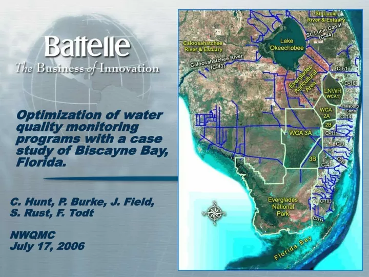
Optimization of water quality monitoring programs with a case study of Biscayne Bay, Florida. C. Hunt, P. Burke, J. Field, S. Rust, F. TodtNWQMCJuly 17, 2006
Project Background • SFWMD Governing Board and District Management Team requested optimization of monitoring program • Contracted with Battelle in Dec. ’04 to: • Evaluate previous optimization efforts of the regional water quality network; and • Statistically optimize the remainder of the network not yet reviewed (projects that acquire Type II andTypeIII Mandated data) • Assembled team of District lead scientists and program/project managers to oversee technical aspects of project (DOTT)
What is optimization? • Literature review for SFWMD on environmental optimization • Found ~10 articles directly address environmental measurement optimization • More publications are in network design field • Some attributes of optimization • Degree that sampling, laboratory analysis, and resources can be trimmed without losing key statistical information • Accurate assessment of quality over time and trends or other changes at individual locations (or a geographic domain) • Removing redundancy in measurement program • Spatial correlation • Temporal (autocorrelation) • Parameter (more than one measure of the same process or WQ condition) • Relocation or adding or both to maximize spatial/temporal scale sampling
How is optimization approached? • Historically tended to use experience, intuition and subjective judgment (Ning and Chang 2002) • Recently approaches • EPA DQO process • Geospatial statistics • Kriging (spatial) • Statistical models (temporal and spatial) • Seasonal Kendal Tau, Spatial Kendal Tau • Time series and probabilistic frameworks/models to look at structural discrepancy between models with the autoregressive distance estimator. • Software based packages • PNNL/EPA Visual Sample Plan (VSP) • Others
What was our approach for the SFWMD? • 2004 EPA DQO Guidance for the Data Quality Objectives Process. http://www.epa.gov/quality/qs-docs/g4-final.pdf • Clearly define the problem so that the focus of the study will be clear and unambiguous • Define the decision that will be resolved using data to address the problem • Identify the informational inputs that will be required to resolve the decision • Specify the spatial and temporal circumstances that are covered by the decision • Integrate the outputs from previous steps into a single statement that describes the logical basis for choosing among alternativeactions • Specify acceptable limits on decision errors to establish appropriate performance goals for limiting uncertainty in the data • Identify the most resource-effective sampling and analysis design for generating data that satisfy the DQOs
What did we do? • Defined project objectives and goals, described all data uses, and determined the management and policy decisions the data will support. • Ensured data used for statistical analyses were appropriate, complete, and accurate. • Defined geographic domains and whether the data for individual sites or geographic regions were to be evaluated • Developed a Power Analysis Procedure For Trend Detection With Accompanying SAS Software (Steve Rust, Columbus) • Addressed seasonal trends and autocorrelation to ensure statistical results are not overstating the power of the monitoring to detect trends. • Applied the power analysis to alternative monitoring designs.
Optimization Project Overview • 5 of 25 projects removed through data use evaluation • 1 removed due to no identifiable end users • 4 projects consolidated into two projects for analysis • 17 projects evaluated in detail • 364 sampling locations • 1.4 million records
Statistical methods • Monte Carlo simulations using the Seasonal Kendall Tau Test for Trend • Nonparametric Sign Test: simulation experiments to assess the power to detect changes in a parameter's distribution from a target value • Spearman's rank correlation: non-parametric version of the Pearson Product Moment correlation analysis to evaluate correlations between stations • Wilcoxan rank sum test: to examine similarities and degree of covariance between specific stations • PCA analysis • SAS PROC CLUSTER, Ward method
Power Analysis Procedure For Trend Detection With Accompanying SAS Software • Mixed model fitted to the data (Yt = α + β(t-t0) + St + ε1 + ε2) • Fits data to form a basis for generating simulated water quality parameter data to support a Monte Carlo based power analysis procedure • Generate multiple replicate simulated water quality time series data sets • Perform a Seasonal Kendall’s Tau trend analysis procedure for each simulated time series data set • Gives a point estimate of the slope vs. time for the log-transformed water quality parameter values • Estimate the annual proportion change (APC) in water quality parameter values that is detectable with 80% power using a simple two-sided test based on the slope estimate performed at a 5% significance level • Seasonal Kendall Tau Test for Trend
Biscayne Bay Case Study • Two Water Quality programs • DERM: Canals and Bay • FIU: Bay • Stations • FIU (16 parameters, monthly) • 35 Bay • DERM (22 parameters, monthly) • 72 canal stations • 41 Bay • Similar goals and data uses (sort of) • Not coordinated in time • Partial overlap in space (x, y, z)
Biscayne Bay Case Study • Similar parameters • Different laboratories • Limited optimization to five (5) parameters • Examined parameter level correlation to remove those that are high correlated and that were considered redundant
BISC ProjectPurpose • Ensure long-term trends can be detected under various climatic cycles, events, and watershed changes at spatial and temporal scales characteristic of the system. • Enable documentation of changes in water quality resulting from comprehensive storm water improvement programs. • Ensure any design changes can adequately measure changes resulting from alterations in freshwater source strengths and hydrological changes. • Support development of non-degradation criteria development
BISC Key data uses • Biscayne Bay Minimum Flows and Levels • CERP Implementation (Biscayne Bay Coastal Wetlands Project, C-111 Spreader Project, Wastewater Reuse Project, RECOVER Monitoring and Assessment Plan) • Water Reservations (under Acceler8 and CERP) • Clean Water Act (TMDL development) and Florida Statues (373.4595), mandates for protecting Outstanding Florida Waters (non-degradation standard) and tracking trends. • Biscayne Bay Swim Plan
Goals of the BISC optimization • Evaluate the FIU and DERM Biscayne Bay data together to identify spatial, temporal, and parameter redundancies/data gaps • Statistically identify geographic domains such as near shore stations, mid-bay stations, and offshore stations • Recommend potential program optimization scenarios for the geographic domains to include: • addition or remove parameters • removal, addition or rearrangement station locations • modification of sample collection frequency
Objectives of the BISC optimization • To determine inter-laboratory data comparability • To determine redundancy among optimization parameters by major geographic domains • To determine spatial redundancy among the stations sampled by major geographic domains • To determine trend detect by major geographic domains • To recommendation changes to the sampling program • Required development of alternatives designs
BISC Optimization Approach taken to address these • Inter-laboratory comparability • Congruent stations, 2 types (same location; nearby) • Statistical steps • Box plots • Scatter plots • Temporal plots • Geospatial domains • Biscayne Bay regions • 11 canals discharging to the coastal domain • Statistical analysis (Bay only) • Box plots • Cluster analysis • Trend analysis
Biscayne Bay Inter-laboratory Comparison • Sampling depth matches were not consistently possible • Sampling times did not match up well
BISC Optimization Inter-Laboratory Stations and parameters compared • Comparison data selected as any sample from the surface (<0.5m depth) and from 3 ±0.9 m depth within a 24 hour time window.
BISC Optimization Lab Inter-comparison – Box plots • Salinity: surface • Dissolved Oxygen: 3±0.9m
BISC Optimization Lab Inter-comparison – Box plots SurfaceAmmonia Surface TPO4
Lab Inter-comparison – Conclusions • Ammonia data is not comparable due to method differences • Salinity, dissolved oxygen, TPO4 data can be combined for optimization
Geographic Domain Determination • SAS PROC CLUSTER, WARD Procedure • Quarterly aggregated salinity and temperature from <0.5 m depth for each station • 46 quarterly periods from Winter 1992 through Spring 2003 • Used the time period with the highest number of stations • 12 time periods from Spring of 2000 through winter 2003 • Clustering on 24 variables • 2 parameters times 12 time periods
Geographic Domains: • Five geographic domains based on the 15 clusters that explain 81 percent of the variability • Similar to those found by Caccia and Boyer (2005) using more sophisticated procedures
Potential redundancies among stations • Cluster output was also used to identify potentially redundant station pairs • Paired stations had to be in close proximity. • Underlined stations were excluded for spatial alternatives analysis since the data from these stations.
Alternatives used for optimization • Spatial Alternative 1: DERM program design only by geographic domain • Spatial Alternative 2: FIU program design only by geographic domain • Spatial Alternative 3: RECOVER MAP stations only by geographic domain. • Spatial Alternative 4: Northern BB and Offshore Central BB redundant stations removed • other geographic domains not evaluated due to few redundant stations. • Temporal Alternative 1: Base case – monthly sampling • Temporal Alternative 2: Base case – bi-monthly sampling
TPO4 Intermediate Biscayne Bay geographic domain Statistical outputsModel output vs actual data • Data aggregation • All stations in a geographic domain • 15-day windows • Combined programs • 1994 through 2003
ANNUAL PROPORTION CHANGE DETECTABLE (percent) • TPO4 with 80% power and p =0.05 for base and alternative monitoring designs
ANNUAL PERCENTAGE CHANGE DETECTABLE (percent) • Salinity with 80% power and p =0.05 for base and alternative monitoring designs
Conclusions • Large range in the APC in trend detection • Smallest: TPO4 and TOTN • Highest: salinity • Intermediate: dissolved oxygen and chlorophyll • Highest salinity APC: Northern, West Central and Southern Biscayne Bay • these geographic domains have the highest data variability • Several stations in the combined program likely provide redundant data. • Removal for trend detection does not greatly affect the APC except for salinity in the Northern Bay. • Decreasing temporal sampling • monthly sampling slightly increases the APCs • bi-monthly increases the APC more • Decreased sampling interval for salinity in highly variable areas show large increases in APC
Conclusions (Continued) • Modifications to the sampling programs possible • Depend greatly on the level of change that needs to be detected and the time frame over which the change must be observed • TPO4 and TOTN temporal monitoring could be reduced • Detecting salinity changes will require more extensive sampling in highly variable locations • Relocation some stations into the highly variable West Central Bay may improve ability to detect trends in salinity
Kissimmee River Eutrophication Abatement (KREA) Project • Inventory the water quality in tributaries discharging into pools A-E of C-38 and in the S154 basin entering Lake Okeechobee south of pool E • Provide monitoring data to assess the efficacy of Best Management Practices (BMPs) for reducing phosphorous in surface discharge from dairies • Monitor phosphorous contributions from each tributary • Estimate phosphorous loads leaving Lake Okeechobee watershed basins • Identifying high episodic phosphorous events and locating corresponding source areas
Kissimmee River Eutrophication Abatement (KREA) Project • Four primary parameters were selected (DO, TKN, TPO4 and CL). • Power analyses for each station-parameter combination were performed using the following power analysis steps: • Fit a statistical model to the water quality parameter data to have a basis for generating simulated data to support a Monte Carlo based power analysis procedure • Generate multiple replicate simulated water quality time series data sets; for all power analyses reported here, each time series generated was for a 5-year monitoring period • Perform a Seasonal Kendall’s Tau trend analysis procedure for each simulated time series data set; in particular, obtain a point estimate of the slope vs. time for the log-transformed water quality parameter values • Estimate the annual proportion change (APC) in water quality parameter values that is detectable with 80% power using a simple two-sided test based on the Seasonal Kendall’s Tau slope estimate performed at a 5% significance level • Parameter values were natural log-transformed for statistical modeling with • Fixed seasonal effects that repeat themselves in an annual cycle • A long-term linear trend in the log-transformed parameter concentrations; this corresponds to a fixed percentage increase or decrease in the water quality parameter each year • A random error term representing temporal variability in true water quality parameter values; these error terms are allowed to be correlated from one time point to the next in order to capture any serial autocorrelation that is present in the monitoring data • A random error term representing sampling and chemical analysis variability; these error terms are assumed to be stochastically independent from one time point to the next
TPO4 concentrations - KREA • Tributary stations • TPO4 time series data for all stations except stations 04 and 22 exhibit significant serial autocorrelation • Detectable APC values for tributary stations other than 20, 25, and 30A at the current monitoring frequency of 24 samples per year are in the range of 21%-50% • Reducing sampling frequencies has smaller than expected effect on detectable APC values since there is significant autocorrelation exhibited in the TPO4 time series data • River channel stations • TPO4 time series data for all stations except station 91 exhibit significant serial autocorrelation • Detectable APC values for stations 93, 95 and 98 are considerable larger than those for other KREA tributary stations due to the fact that these stations exhibit the highest levels of variability and serial autocorrelation • Detectable APC values for river channel stations other than 93, 95 and 98 at the current monitoring frequency of 12 samples per year are in the range of 16%-33% • Reducing sampling frequencies has smaller than expected effect on detectable APC values since there is significant autocorrelation exhibited in the TPO4 time series data
Monitoring Historic Monitoring in the past was frequently conducted independently from other planning or management activities (i.e. context was not always understood). • Compliance - to establish whether or not a pollutant source is meeting requirements of a permit or regulation (e.g., individual plant or source) • Fate and transport - assessment of pollution conditions and transport pathways • Ecological effects - measurement of responses to detect ecological consequences • Human health effects - measurement of indicators of human exposure potential or human response • Trend - evaluates changes through time
Monitoring Overview Monitoring in the past was frequently conducted independently from other planning or management activities (i.e. context was not always understood). • Compliance - to establish whether or not a pollutant source is meeting requirements of a permit or regulation (e.g., individual plant or source) • Fate and transport - assessment of pollution conditions and transport pathways • Ecological effects - measurement of responses to detect ecological consequences • Human health effects - measurement of indicators of human exposure potential or human response • Trend - evaluates changes through time
Developing and Implementing Effective Assessment and Monitoring Programs • Managing Troubled Waters (1990) US National Research Council • Monitoring Guidance for the National Estuary Program (1992) US EPA 842-B-92-004 http://www.epa.gov/OWOW/estuaries/guidance/contents.html • Managing Wastewater in Coastal Urban Areas (1993) US National Research Council
Commonalty among the Guidance in these Documents • Early, interactive planning • Understanding and defining expectations • Goal setting • Use of historical information • Assessment of current status • Research to fill knowledge gaps • Monitoring to assess status and progress • Statistical validity in study design • Data management plan • Dissemination of information • Feedback and redesign
Monitoring Today Fundamental component of an environmental management system (National Research Council 1990) “The range of activities needed to provide management information about environmental conditions or contaminants.” Conceptual Models (How does the system work?) Modeling (Numeric, statistical) Laboratory and field research Preliminary or scoping studies Time-series measurements Data analysis, synthesis, and interpretation Production and dissemination of information
Monitoring Today “.. integrated and coordinated with a specified goal of producing predefinedmanagementinformation.” • “… the sensory component of environmental management.” • Included in an integrated approach that encompasses: • Compliance • Fate and transport • Ecological effects • Human health effects • Trend assessment • Decision making • Communication
Conceptual Ecological Model pertaining to influences of erosion and sedimentation on water quality in a typified shallow aquatic system.
Conceptual Ecological Model pertaining to influences of erosion and sedimentation on water quality in a typified shallow aquatic system.