Download
1 / 20
200 likes | 224 Vues
Distributed Process Scheduling: A System Performance Model. Vijay Jain CSc 8320, Spring 2007. Outline. Overview Process Interaction Models A System Performance Model Efficiency Loss Processor Pool and Workstation Queuing Models Comparison of Performance for Workload Sharing References.

E N D
Distributed Process Scheduling: A System Performance Model Vijay Jain CSc 8320, Spring 2007
Outline • Overview • Process Interaction Models • A System Performance Model • Efficiency Loss • Processor Pool and Workstation Queuing Models • Comparison of Performance for Workload Sharing • References
Overview • Before execution, processes need to be scheduled and allocated with resources • Objective • Enhance overall system performance metric • Process completion time and processor utilization • In distributed systems: location and performance transparency • In distributed systems • Local scheduling (on each node) + global scheduling • Communication overhead • Effect of underlying architecture
Process Interaction Models • Precedence process model: Directed Acyclic Graph (DAG) • Represent precedence relationships between processes • Minimize total completion time of task (computation + communication) • Communication process model • Represent the need for communication between processes
Process Interaction Models • Optimize the total cost of communication and computation • Disjoint process model • Processes can run independently and completed in finite time • Maximize utilization of processors and minimize turnaround time of processes
Communication overhead Process Models Partition 4 processes onto two nodes
System Performance Model Attempt to minimize the total completion time of (makespan) of a set of interacting processes
System Performance Model (Cont.) • Related parameters • OSPT: optimal sequential processing time; the best time that can be achieved on a single processor using the best sequential algorithm • CPT: concurrent processing time; the actual time achieved on a n-processor system with the concurrent algorithm and a specific scheduling method being considered • OCPTideal: optimal concurrent processing time on an ideal system; the best time that can achieved with the concurrent algorithm being
System Performance Model (Cont.) considered on an ideal n-processor system (no interprocessor communication overhead) and scheduled by an optimal scheduling policy • Si: ideal speedup obtained by using a multiple processor system over the best sequential time • Sd: the degradation of the system due to actual implementation compared to an ideal system
System Performance Model (Cont.) Pi: the computation time ofthe concurrent algorithm onnode i (RP 1)
System Performance Model (Cont.) (The smaller, the better)
System Performance Model (Cont.) • RP: Relative processing • Shows how much loss of speedup is due to the substitution of the best sequential algorithm by an algorithm better adapted for concurrent implementation but which may have a greater total processing need • Sd • Degradation of parallelism due to algorithm implementation
System Performance Model (Cont.) • RC: Relative concurrency • How far from optimal the usage of the n-processor is • RC=1 best use of the processors • : Efficiency Loss is loss of parallelism when implemented on a real machine. • can be decomposed into two terms: = sched + syst
Efficiency Loss Impact factors: scheduling, system, and communication
Workload Distribution • Performance can be further improved by workload distribution • Load sharing: static workload distribution • Dispatch process to the idle processors statically upon arrival • Corresponding to processor pool model • Load balancing: dynamic workload distribution • Migrate processes dynamically from heavily loaded processors to lightly loaded processors • Corresponding to migration workstation model
Workload Distribution • Performance of systems described as queuing models can be computed using queuing theory. An X/Y/c queue is one where: • X: Arrival Process, Y: Service time distribution, c: Numbers of servers • : arrival rate; : service rate; : migration rate • : depends on channel bandwidth, migration protocol, context and state information of the process being transferred.
Processor-Pool and Workstation Queueing Models Static Load Sharing Dynamic Load Balancing M for Markovian distribution
Comparison of Performance for Workload Sharing (Communication overhead) (Negligible Communication overhead) =0 M/M/1=M/M/2
References • “Distributed Operating Systems and Algorithms” by Randy Chow and Theodore Johnson • “Opearting System Concepts” by Silberschatz, Galvin and Gagne • “Time Comparative Simulator for Distributed Process Scheduling Algorithms”, Transactions on Engineering, Computing and Technology Volume 13 May 2006 ISSN 1305-5313, Nazleeni Samiha Haron, Anang Hudaya Muhamad Amin, Mohd Hilmi Hasan, Izzatdin Abdul Aziz,and Wirdhayu Mohd Wahid